容器服务
容器服务


文档指南

请输入


- 文档首页
 容器服务AI 云原生训练套件veRL Code Sandbox 代码生成强化学习
 复制全文
复制全文 下载 pdf
veRL Code Sandbox 代码生成强化学习
 文档反馈
文档反馈 问问助手
问问助手简介
在 R1 模型之后,基于强化学习的代码生成最近取得了显著进展,其中模型通过与代码执行环境交互来学习和改进。然而,直接执行由 LLM 生成的代码带来了安全性风险,因为这些代码可能包含恶意或不稳定的指令,对宿主系统构成威胁。为了解决这一关键问题,Code Sandbox 技术应运而生。它为代码执行提供了一个安全、隔离的环境,有效防止了潜在的危害,并确保了实验的可控性和可重复性。这种方法不仅保障了底层系统的安全,还为评估和提升模型的代码生成能力(例如在经典的 Livecodebench/ HumanEval 代码能力测试基准上)提供了可靠的平台。
在 RL 训练流程中的 rollout 阶段,需要大规模并行执行生成的代码片段以收集经验。火山 veFaas Code Sandbox 的设计充分考虑了高并发需求,能够支持百万核超低延迟(150ms)弹性伸缩能力,实现了高效的 rollout 并发。这种弹性能力使得系统可以根据训练负载动态调整沙箱数量,对于加速 RL 训练、提高 GPU 利用率和整体训练吞吐有较大价值。
本文档为算法工程团队在强化学习训练场景中,使用分布式强化学习框架(veRL+Ray)提供基于火山引擎 VKE 集群的多节点训练环境部署方案,详细指导集群配置、存储卷创建、KubeRay 与 RayCluster 部署等步骤,并在 Eurus-2-RL-Data 数据集上 PPO 微调 Qwen2.5-7B-Instruct-1M 模型 ,并提供数据集处理、任务提交及监控的全流程操作。
本文使用的训练框架 veRL(Volcano Engine Reinforcement Learning for LLMs),是云平台针对大语言模型(LLMs)的强化学习框架。它不仅具备灵活、高效且可扩展的强化学习训练,还提供了名为“HybridEngine”的框架,该框架将控制流(在单进程中运行)与计算流(在分布式多进程中运行)分离,并且可以支持多种计算后端、训练与推理并行策略和性能优化技术。
前置条件
创建高性能计算集群
注意
高性能集群所在的可用区需要与 VKE 节点的可用区一致。
创建 VKE 集群
配置项 | 说明 |
集群配置 | |
Kubernetes 版本 | 选择 v1.28 及以上版本。 |
容器网络模型 | 选择 VPC-CNI。 |
节点池配置 | |
托管节点池 | 开启 托管节点池。 |
可用区 | 与 高性能计算集群 所在的可用区相同。 |
计算规格 | 由于Qwen2.5-7B-Instruct-1M模型参数较大,因此需要选择有较大显存的 GPU 实例 ,如 ecs.hpcpni3ln.45xlarge 等。 |
高性能计算集群 | 选择之前创建的高性能计算集群。 |
节点数量 | 1个。 |
数据盘 | 选择 1024 GiB 极速型 SSD 盘和本地盘 SSD ,并将 本地盘 SSD 挂载在 /data01 目录下 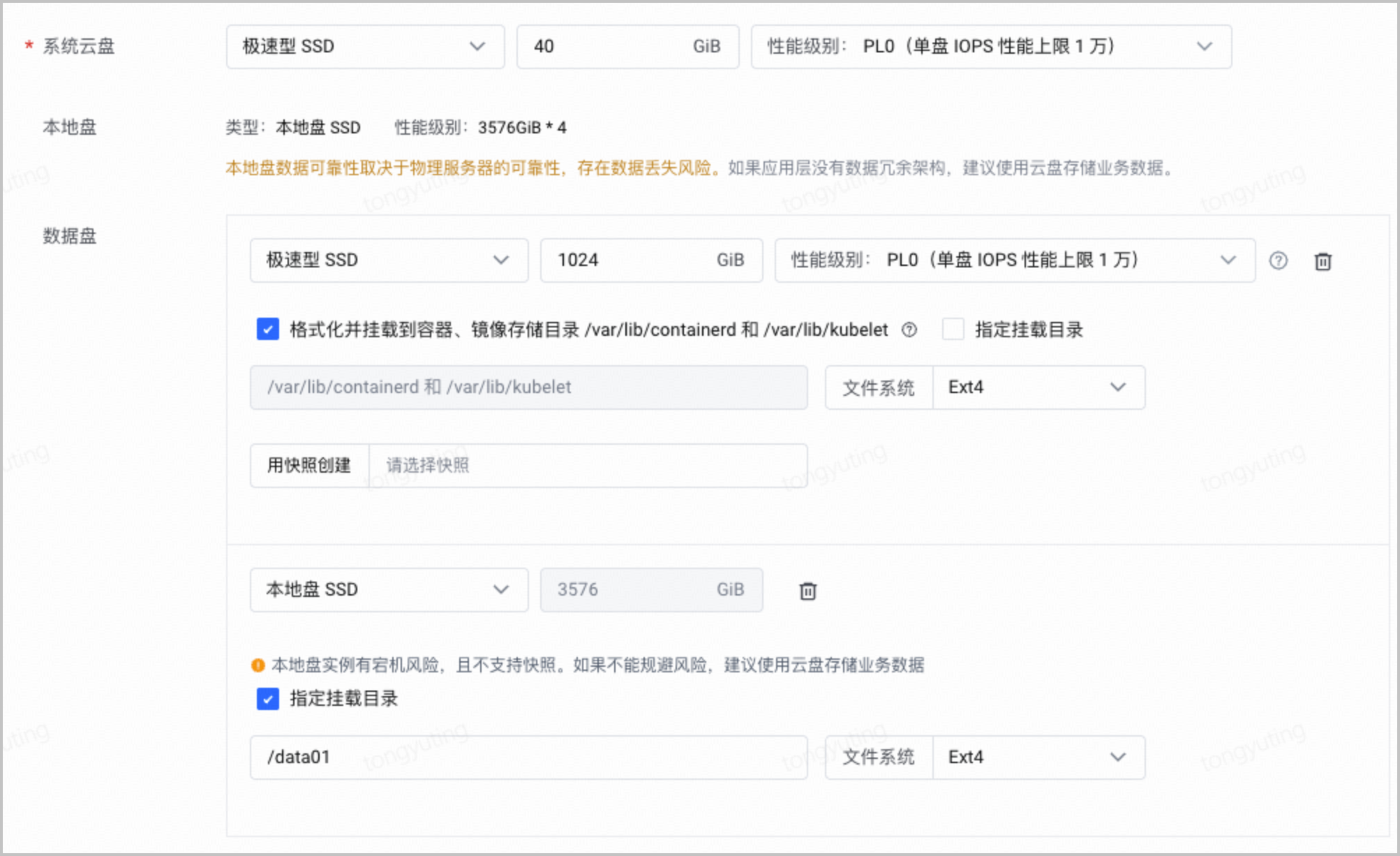 |
组件配置:除了标记为 系统必装 的组件之外,可以根据需要,选择安装以下组件
在 veFaaS 上创建 SandboxFusion 沙箱
创建 API 网关实例
- 登录 API 网关控制台。
- 在左侧导航栏选择 实例管理,在实例管理页面,单击 创建实例。
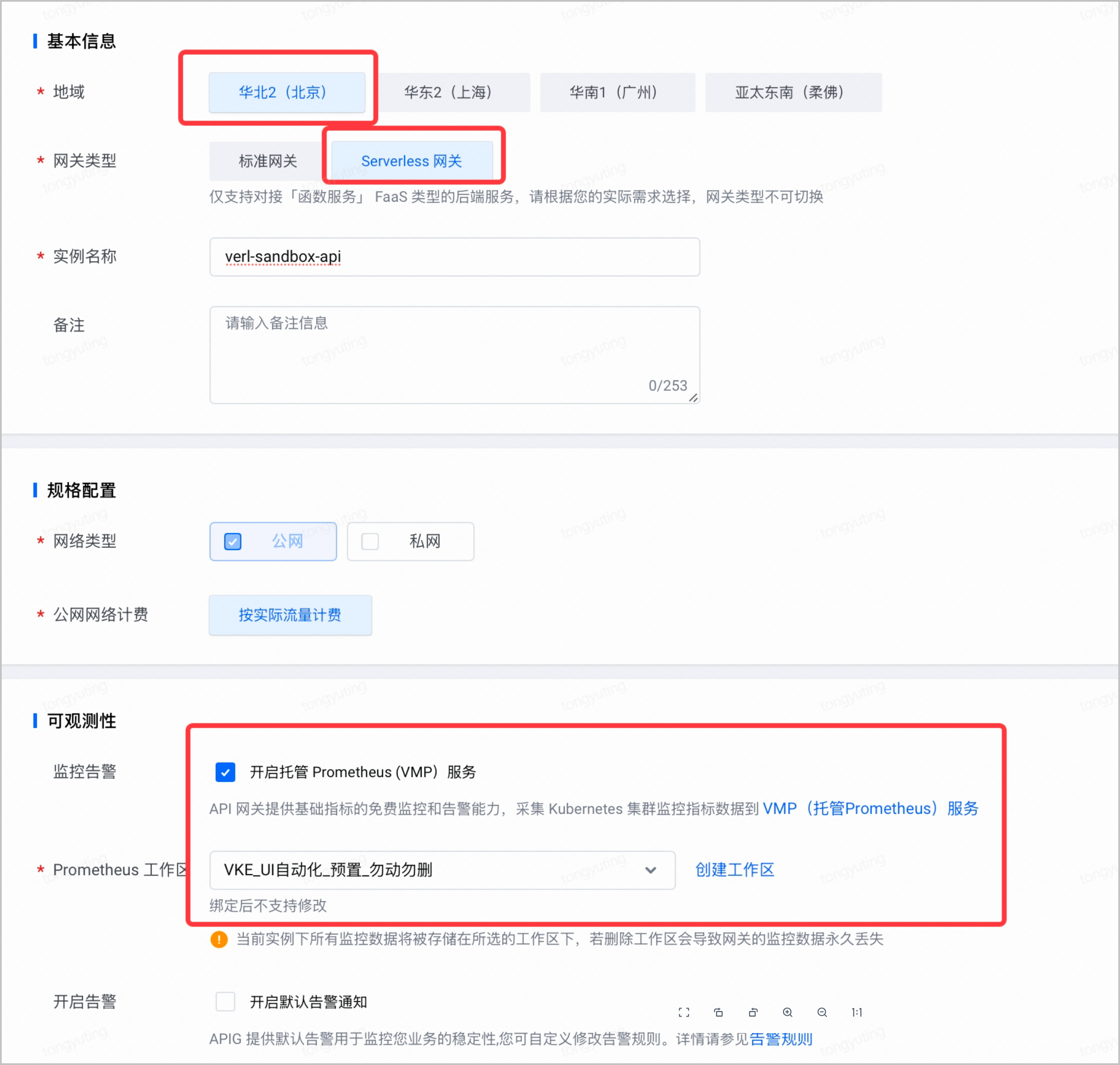
- 地域:选择网关实例所在地域,本例中选择 华北2(北京)。
- 网关类型:选择 Serverless 网关。
- Prometheus 工作区:选择监控实例使用的 VMP 工作区,不需要监控时可以不开启该服务。
-
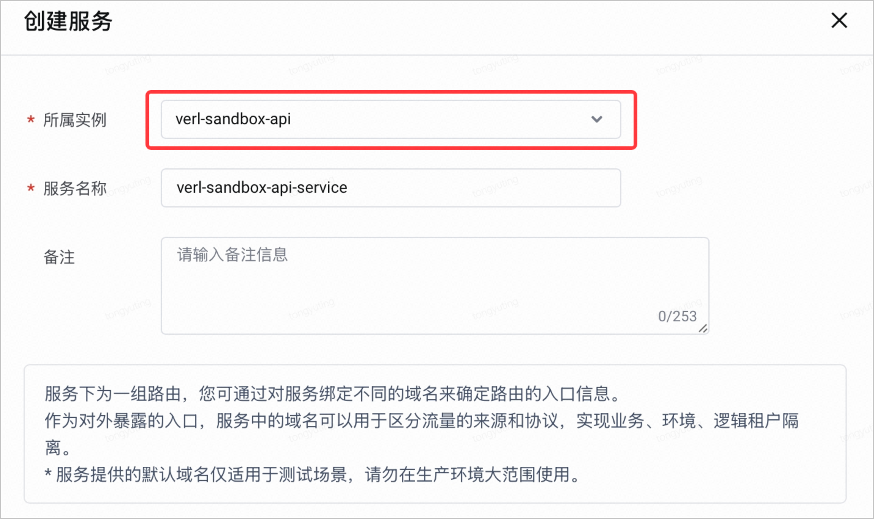
- 在左侧导航栏选择 路由管理 > 服务列表(域名)。单击 创建服务,并关联已创建的 API 网关实例。
-
创建 SandboxFusion 沙箱
- 登录 函数服务控制台。
- 在顶部导航栏,选择目标地域。
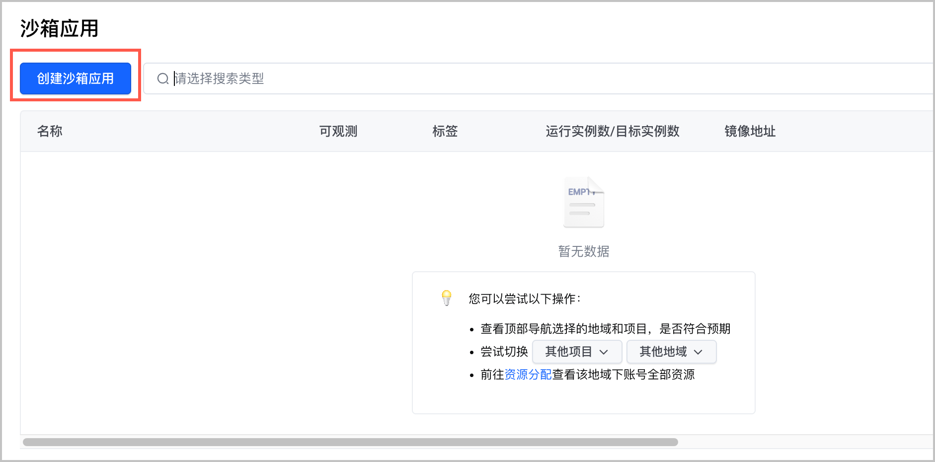
- 在左侧导航栏中选择 云沙箱 > 沙箱应用,单击 创建沙箱应用。
-
- 如下说明,配置沙箱应用参数。完成后,单击 确定,完成配置。
- 配置项配置说明容器镜像
- 选择 公共镜像 中 沙箱类别 为 Code 的镜像。
如有自定义沙箱镜像,,进入 镜像仓库 进行选择。- 启动命令: 默认为bash /root/sandbox/scripts/run.sh,如果是自定义镜像,请按需求改镜像启动脚本。
- 监听端口: 默认为8000,如果是自定义镜像,请按需求修改服务监听端口。
网关路由配置- 域名类型:选择 统一域名。
- 网关实例:选择上一节创建好的 API 网关实例。
- 网关服务:选择上一节创建好的网关服务。
- Path:保持默认/ 即可。
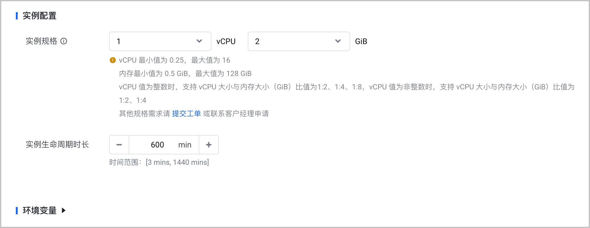
环境变量在默认环境变量的基础上,添加HOME:/home/tiger。高级配置实例规格默认为 1vCPU、2GiB。建议根据需要调整。不启用多并发。
- 单击目标沙箱应用名称,进入沙箱应用详情,选择 沙箱实例 页签,单击 创建沙箱实例,创建云沙箱实例。
-
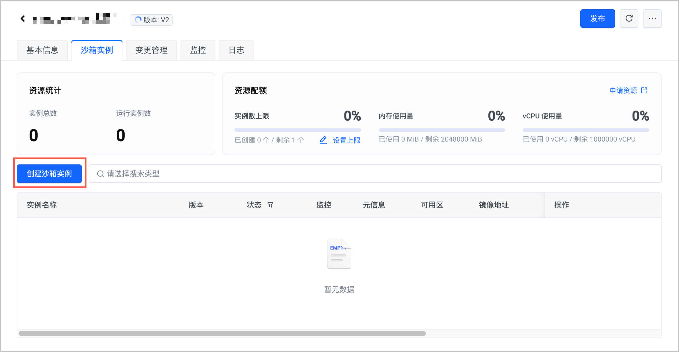
- 配置沙箱实例的存活时长,单位分钟,取值范围为 3min~24*60min,默认 60min,实例自创建起最长可存活 24h。
-
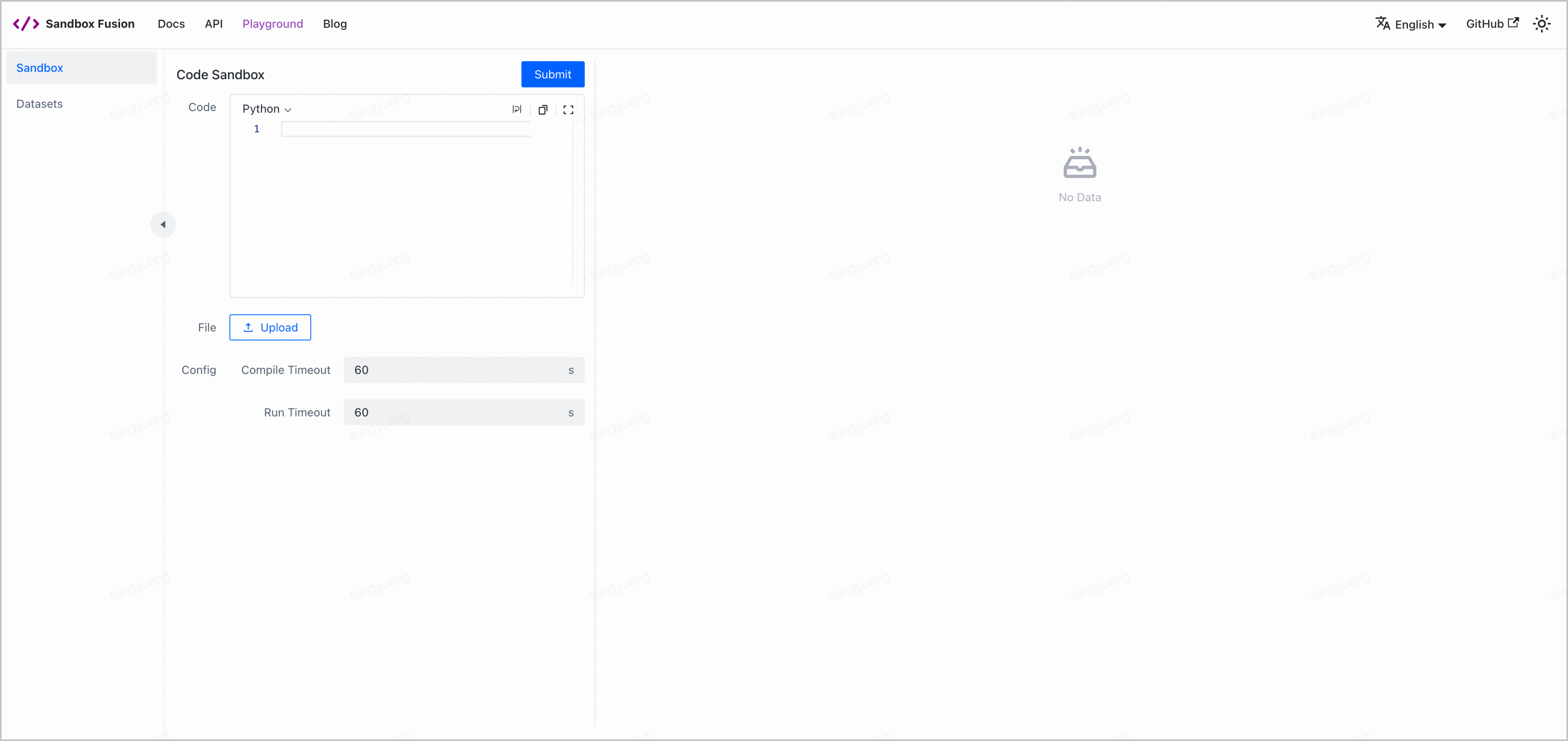
- 创建完成后,选择 基本信息 页面,可以查看沙箱实例的 公网访问 地址信息。单击地址,即可打开 Code Sandbox 代码编辑界面。
-
部署步骤
部署 KubeRay Operator
- 登录 容器服务控制台。
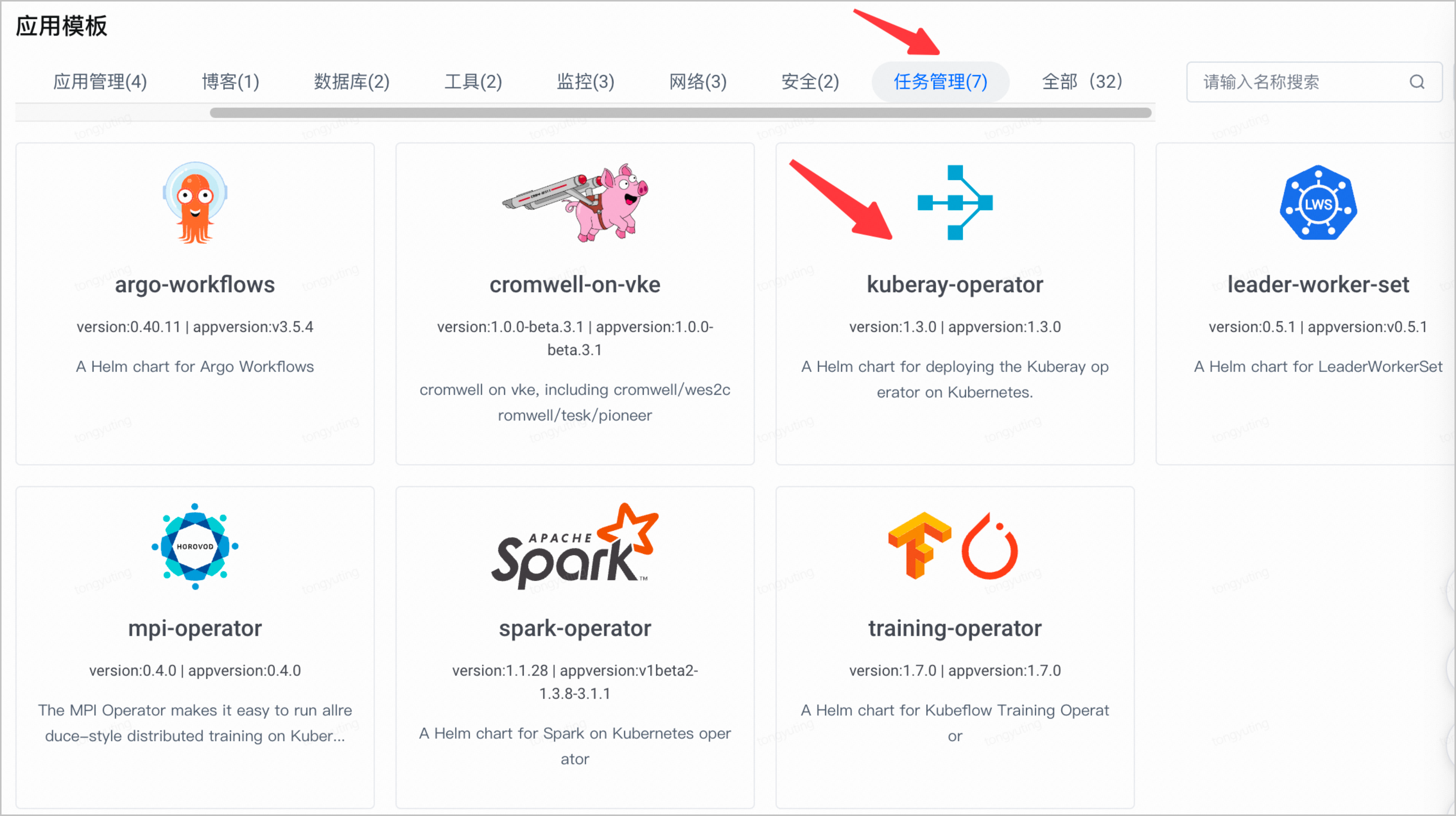
- 在左侧导航栏,选择 应用中心 > 应用模板。
- 在 应用模板 页面,找到 kuberay-operator 应用模板,将鼠标悬停卡片上,单击 部署。
-
- 在 部署应用 页面,配置 kuberay-operator 服务参数。
-
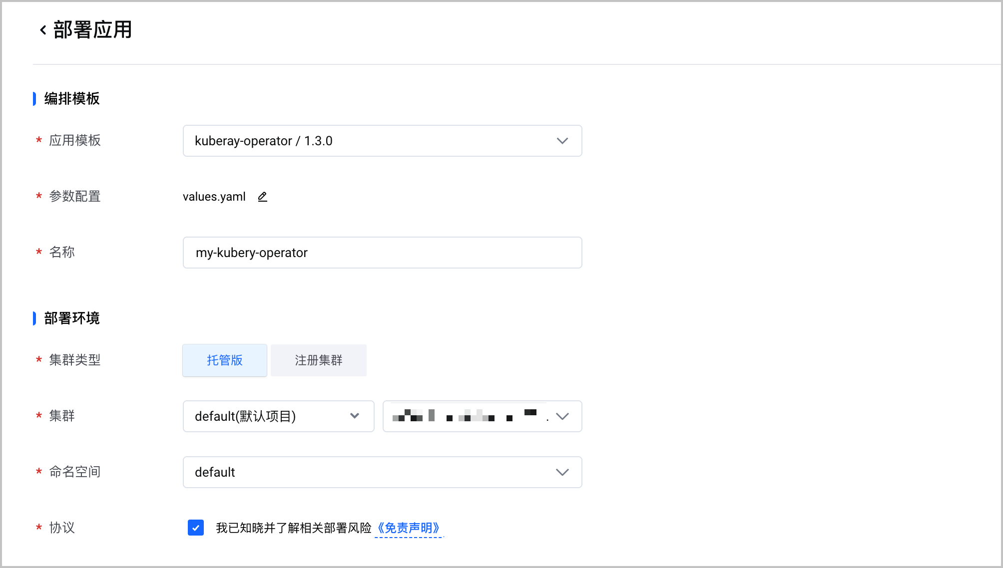
- 参数说明编排模板应用模版选择应用的 Chart 版本,建议选择最新版本。参数配置选择应用的配置方法。每个应用模板的values.yaml文件配置方法不同,详细说明,请参见values.yaml文件中的注释说明。名称设置应用名称,同一个命名空间里名称必须唯一。部署环境集群类型选择集群类型,支持 托管版 和 注册集群。集群命名空间选择目标集群下的命名空间。
- 单击 确定,部署完成应用。
应用部署完成后会显示在 Helm 应用 页面。可进入详情页面查看该应用的基本信息、关联创建的工作负载、服务、其他资源等。

部署 RayCluster
- 按需修改下面的 Yaml 文件内容:
- 根据节点规格修改 Yaml 中 head 和 worker 的资源配置,nvidia.com/gpu配置为节点 GPU 数量,cpu 和 memory 建议在预留部分资源给其他系统组件的情况下,尽量多分配,比如分配节点资源的 80%。requests 和 limits 的值修改为一样即可。
注意
memory 需要设置为 300GB 以上。
- rayStartParams 中 tracing-startup-hook为启动深度观测需要,启动脚本已提供在/workspace/verl/tracing/setup_tracing.py中,只需要执行以下几步就可完成深度观测的启动。(样例配置已包含以下配置,可直接使用)。
- 在启动命令中添加tracing-startup-hook: "tracing.setup_tracing:setup_tracing"。
- 配置环境变量 PYTHONPATH=/workspace/verl就能够完成深度观测的启动,数据会自动上报到 APMPlus。
- 对 worker 和 header 实例添加 annotation instrumentation.apmplus.volcengine.com/inject-python:"true"。
- 为减少系统消耗,还需要配置环境变量 OTEL_PYTHON_DISABLED_INSTRUMENTATIONS=system_metrics 。
- 更多配置项说明,请参见 RayCluster Configuration。
apiVersion: ray.io/v1
kind: RayCluster
metadata:
name: raycluster-kuberay
namespace: default
spec:
headGroupSpec:
serviceType: ClusterIP
rayStartParams:
dashboard-host: "0.0.0.0"
tracing-startup-hook: "tracing.setup_tracing:setup_tracing"
template:
metadata:
annotations:
instrumentation.apmplus.volcengine.com/inject-python: "true"
spec:
containers:
- name: ray-head
image: ai-containers-cn-beijing.cr.volces.com/deeplearning/verl:ngc-th2.6.0-cu126-vllm0.8.4-flashinfer0.2.2-cxx11abi0-custom-v1
imagePullPolicy: IfNotPresent
resources:
limits:
cpu: "60"
memory: 600Gi
nvidia.com/gpu: 8
requests:
cpu: "60"
memory: 600Gi
nvidia.com/gpu: 8
volumeMounts:
- name: log-volume
mountPath: /tmp/ray
- name: models
mountPath: /data/models
env:
- name: PYTHONPATH
value: /workspace/verl
- name: OTEL_PYTHON_DISABLED_INSTRUMENTATIONS
value: system_metrics
volumes:
- name: log-volume
emptyDir: {}
- name: models
hostPath:
path: /data01
type: Directory
- 登录 容器服务控制台,在集群列表中单击目标集群名称,进入集群控制台。
- 在左侧导航栏,选择 工作负载 > 对象浏览器。
- 单击 使用 Yaml 创建,选择 类型 为 自定义,填入修改后 Yaml 后,单击右下角 确定 提交,默认部署到 default 命名空间。
-
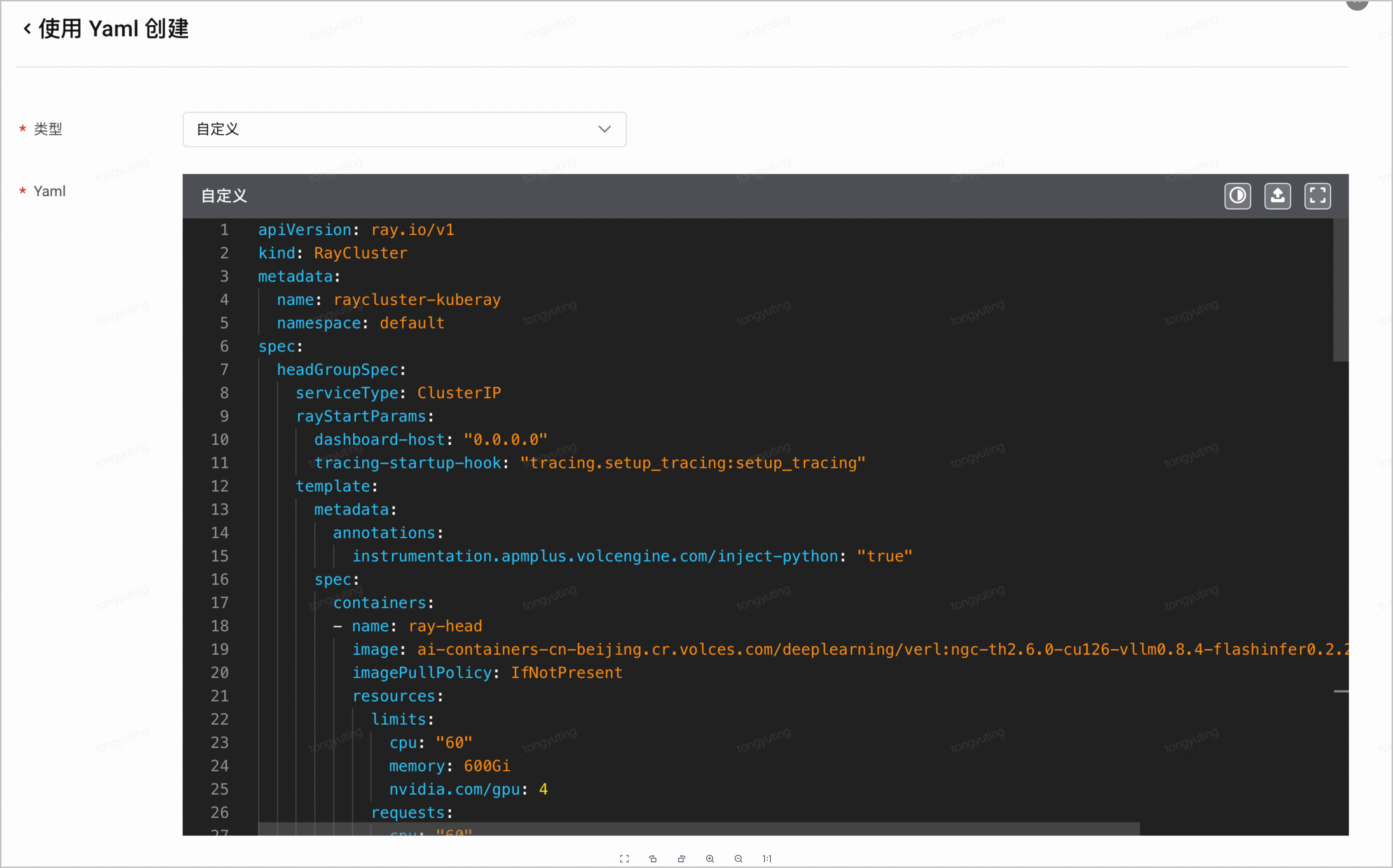
检查运行状态
在左侧导航栏中,选择 工作负载 > 容器组。查看 head 和 worker 容器组的状态(名称分别为 raycluster-kuberay-head-xxxx 和 raycluster-kuberay-workergroup-worker-xxxx),容器组状态显示Running表示完成启动。
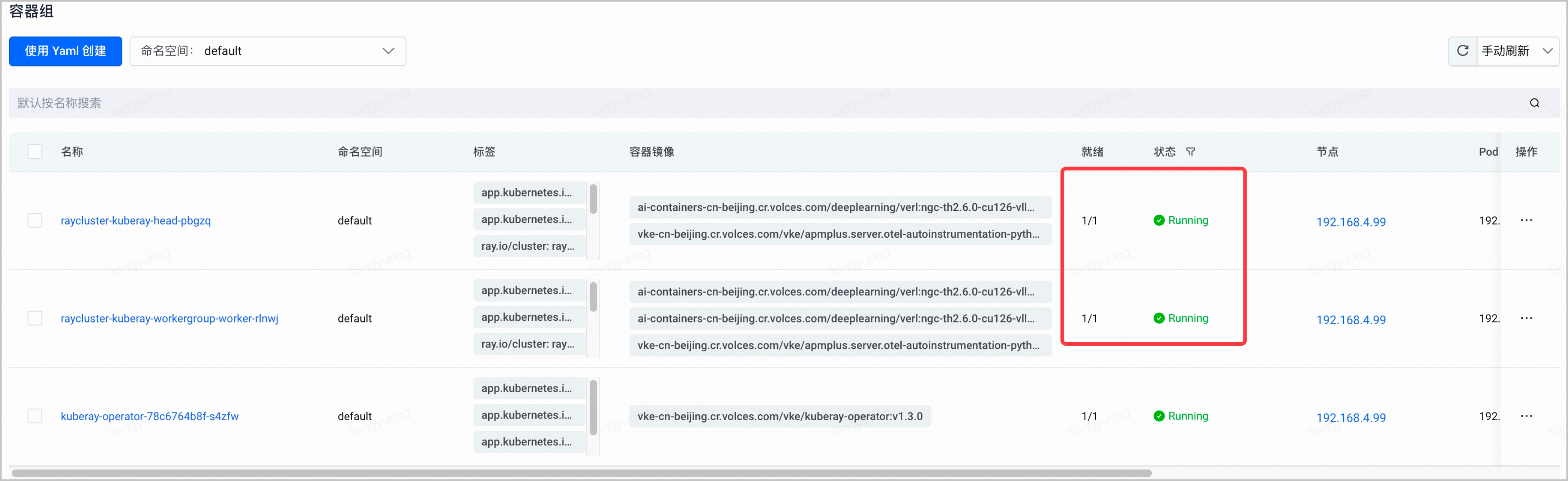
下载模型和数据集
- 在左侧导航栏中,选择 工作负载 > 容器组,单击容器组 raycluster-kuberay-head-xxxx 的名称,进入容器组详情页面,单击右上角 控制台。
-
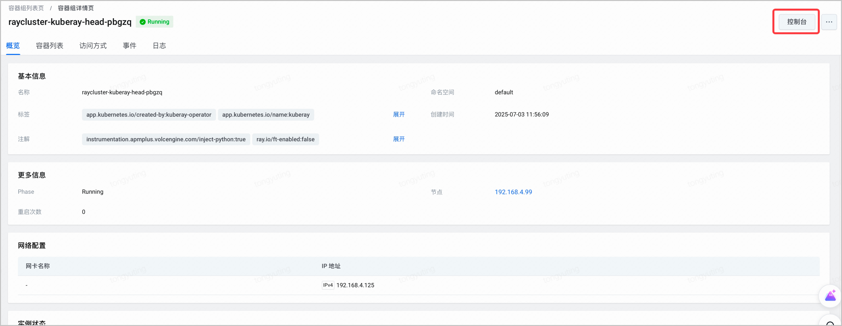
- 在容器组控制台中,执行以下命令,安装 oniond。
export MIRROR_HOST=mirrors.ivolces.com
export DISTRIB="ubuntu jammy"
curl -fsSL https://mirrors.ivolces.com/extra-tools/ubuntu/GPG-KEY-system | gpg --dearmor -o /etc/apt/trusted.gpg.d/volc-extra-tools.gpg
echo "deb [arch=$(dpkg --print-architecture) signed-by=/etc/apt/trusted.gpg.d/volc-extra-tools.gpg] http://mirrors.ivolces.com/extra-tools/ubuntu jammy main" > /etc/apt/sources.list.d/volctools.list && apt update && apt install -y onion-ai-data
- 执行以下命令,进入/data/models目录,下载模型和数据集。
cd /data/models
#下载模型
oniond download model Qwen2.5-7B-Instruct-1M
#下载数据集
oniond download dataset Eurus-2-RL-Data
#实际训练中随机取1000条训练数据作为训练集,创建并执行cut.py,裁剪训练数据集
cd Eurus-2-RL-Data
python cut.py
cut.py
import pandas as pd
# 读取Parquet文件
df = pd.read_parquet('./train.parquet')# 随机提取1000条样本(设置random_state确保结果可重现)
subset_df = df.sample(n=1000, random_state=42)# 保存为新的Parquet文件
subset_df.to_parquet('train1000.parquet')
print(f"已成功随机保存 {len(subset_df)} 条样本到 train1000.parquet")
执行 VKE 本地训练任务
提交训练任务
- 在左侧导航栏中,选择 工作负载 > 容器组,点击 raycluster-kuberay-head-xxxx,点击右上角 控制台。
-
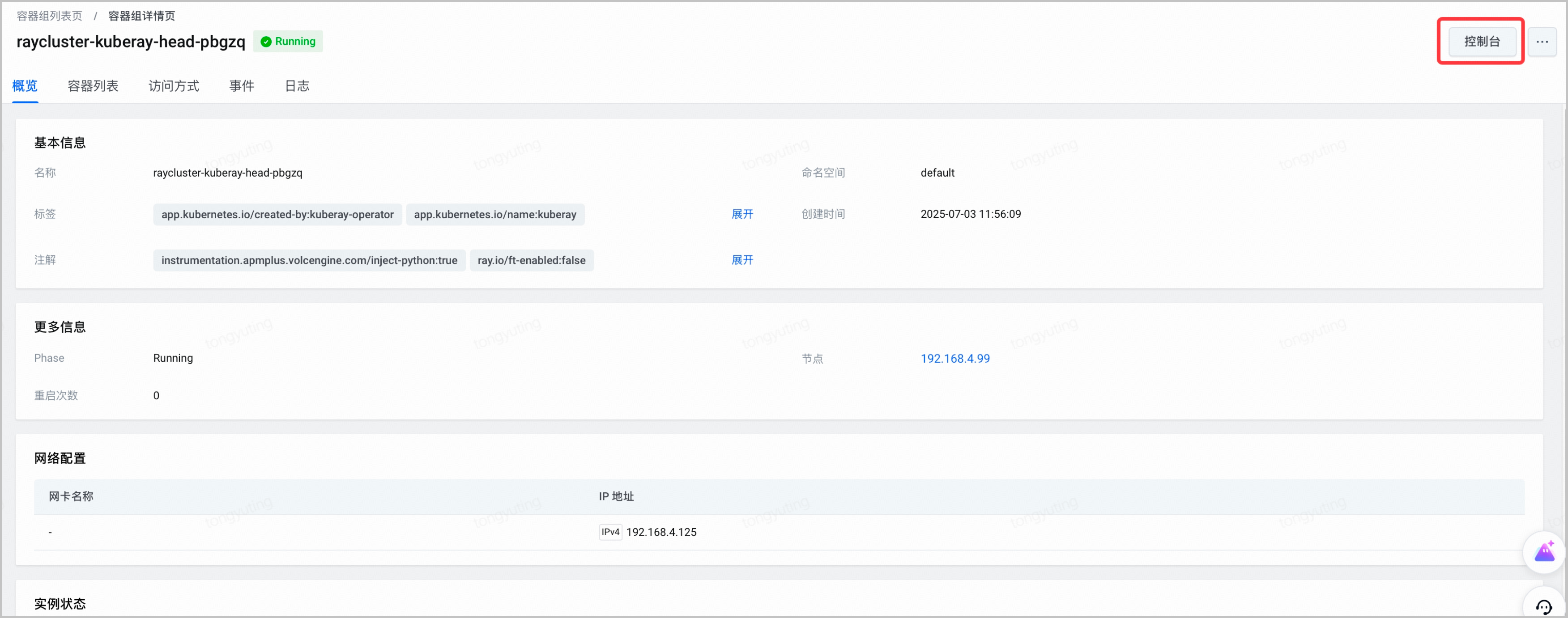
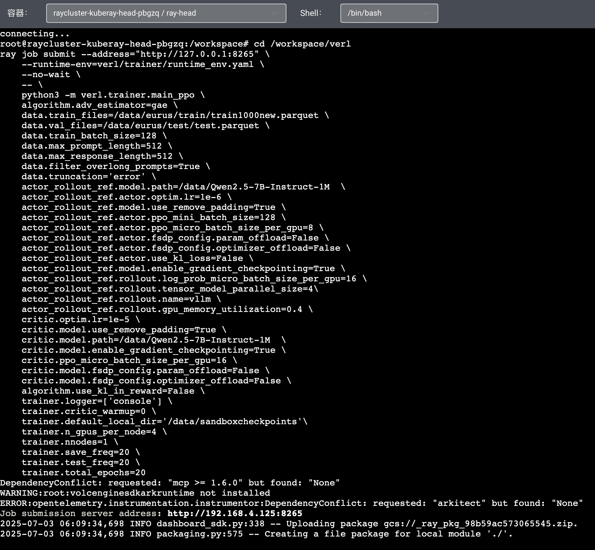
- 在控制台中输入以下命令,进入到 verl 目录,提交训练任务。
- 训练参数的详细说明,请参考:Config Explanation。
- 请将trainer.default_local_dir设置为/data目录内的任意文件夹,即可将训练 checkpoints 保存到指定目录。
- EURUS 数据集中部分样本长度较长,长度超过 512,需要做 filter 处理。
cd /workspace/verl
ray job submit --address="http://127.0.0.1:8265" \
--runtime-env=verl/trainer/runtime_env.yaml \
--no-wait \
-- \
python3 -m verl.trainer.main_ppo \
algorithm.adv_estimator=gae \
data.train_files=/data/models/Eurus-2-RL-Data/train1000.parquet \
data.val_files=/data/models/Eurus-2-RL-Data/validation.parquet \
data.train_batch_size=128 \
data.max_prompt_length=512 \
data.max_response_length=512 \
data.filter_overlong_prompts=True \
data.truncation='error' \
actor_rollout_ref.model.path=/data/models/Qwen2.5-7B-Instruct-1M \
actor_rollout_ref.actor.optim.lr=1e-6 \
actor_rollout_ref.model.use_remove_padding=True \
actor_rollout_ref.actor.ppo_mini_batch_size=128 \
actor_rollout_ref.actor.ppo_micro_batch_size_per_gpu=8 \
actor_rollout_ref.actor.fsdp_config.param_offload=False \
actor_rollout_ref.actor.fsdp_config.optimizer_offload=False \
actor_rollout_ref.actor.use_kl_loss=False \
actor_rollout_ref.model.enable_gradient_checkpointing=True \
actor_rollout_ref.rollout.log_prob_micro_batch_size_per_gpu=16 \
actor_rollout_ref.rollout.tensor_model_parallel_size=4\
actor_rollout_ref.rollout.name=vllm \
actor_rollout_ref.rollout.gpu_memory_utilization=0.4 \
critic.optim.lr=1e-5 \
critic.model.use_remove_padding=True \
critic.model.path=/data/models/Qwen2.5-7B-Instruct-1M \
critic.model.enable_gradient_checkpointing=True \
critic.ppo_micro_batch_size_per_gpu=16 \
critic.model.fsdp_config.param_offload=False \
critic.model.fsdp_config.optimizer_offload=False \
algorithm.use_kl_in_reward=False \
trainer.logger=['console'] \
trainer.critic_warmup=0 \
trainer.default_local_dir='/data/models/localcheckpoints'\
trainer.n_gpus_per_node=8 \
trainer.nnodes=1 \
trainer.save_freq=20 \
trainer.test_freq=20 \
trainer.total_epochs=20
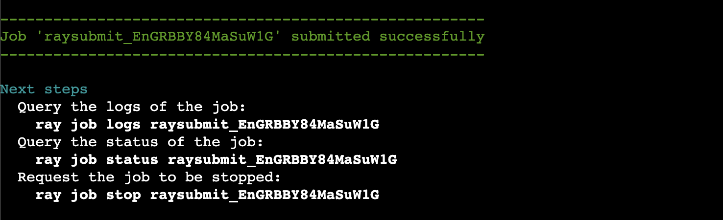
提交成功后,预期输出如下图所示。
查看训练任务状态
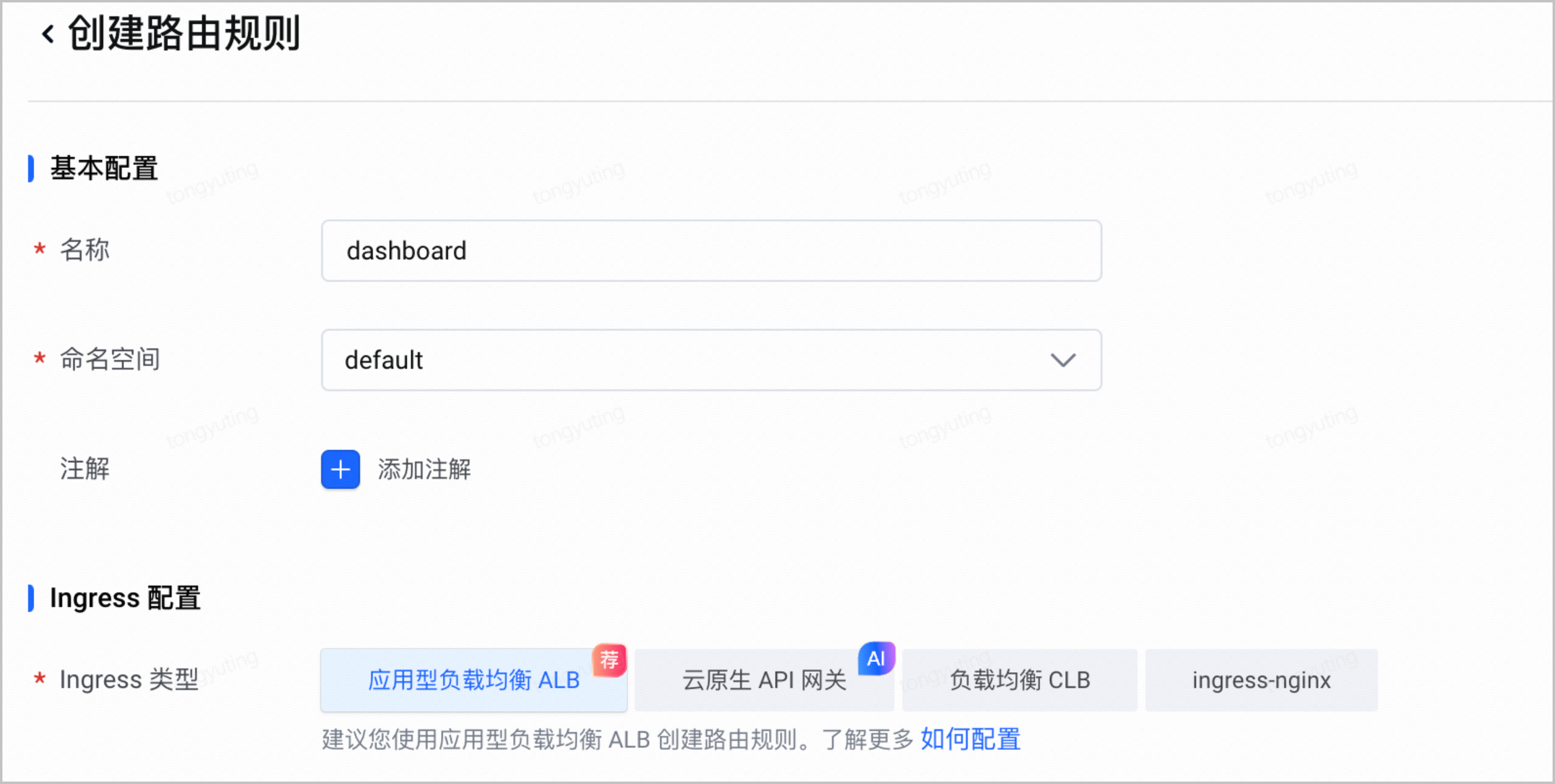
- 在集群页面 服务与路由 > 路由规则,单击 创建路由规则,对外暴露 ray dashboard 服务。
-
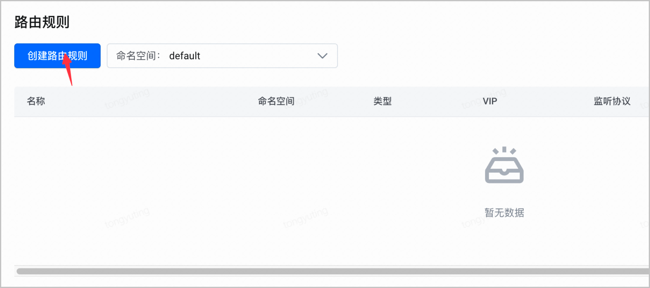
- 配置 ALB Ingress 的详细参数,更多参数说明和详细的操作步骤,请参见 通过控制台创建 ALB Ingress。
-
-
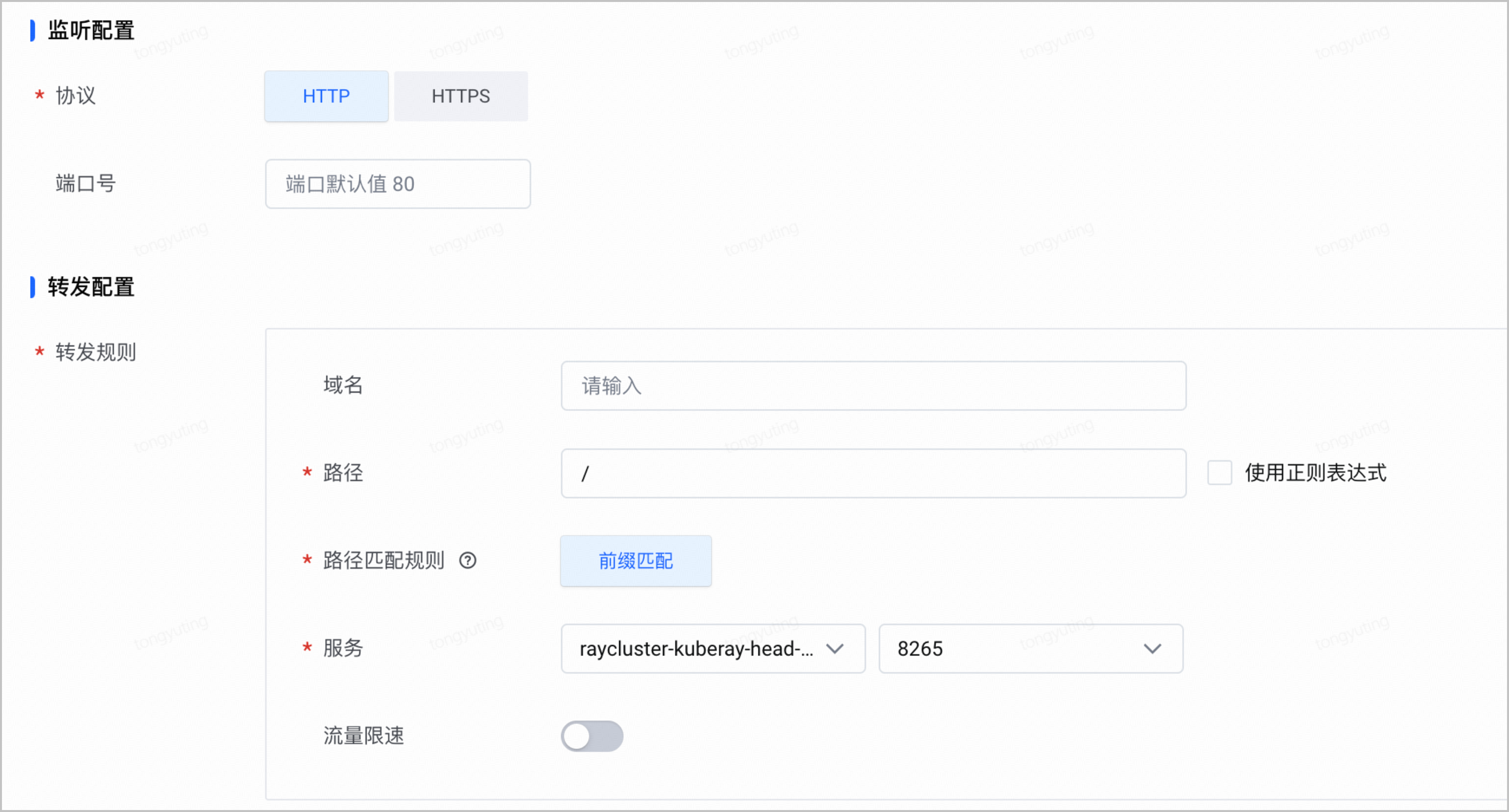
- 配置项说明Ingress类型选择 应用型负载均衡 ALB。协议选择 HTTP。路径输入/。服务选择 raycluster-kuberay-head-xxxxxx : 8265。
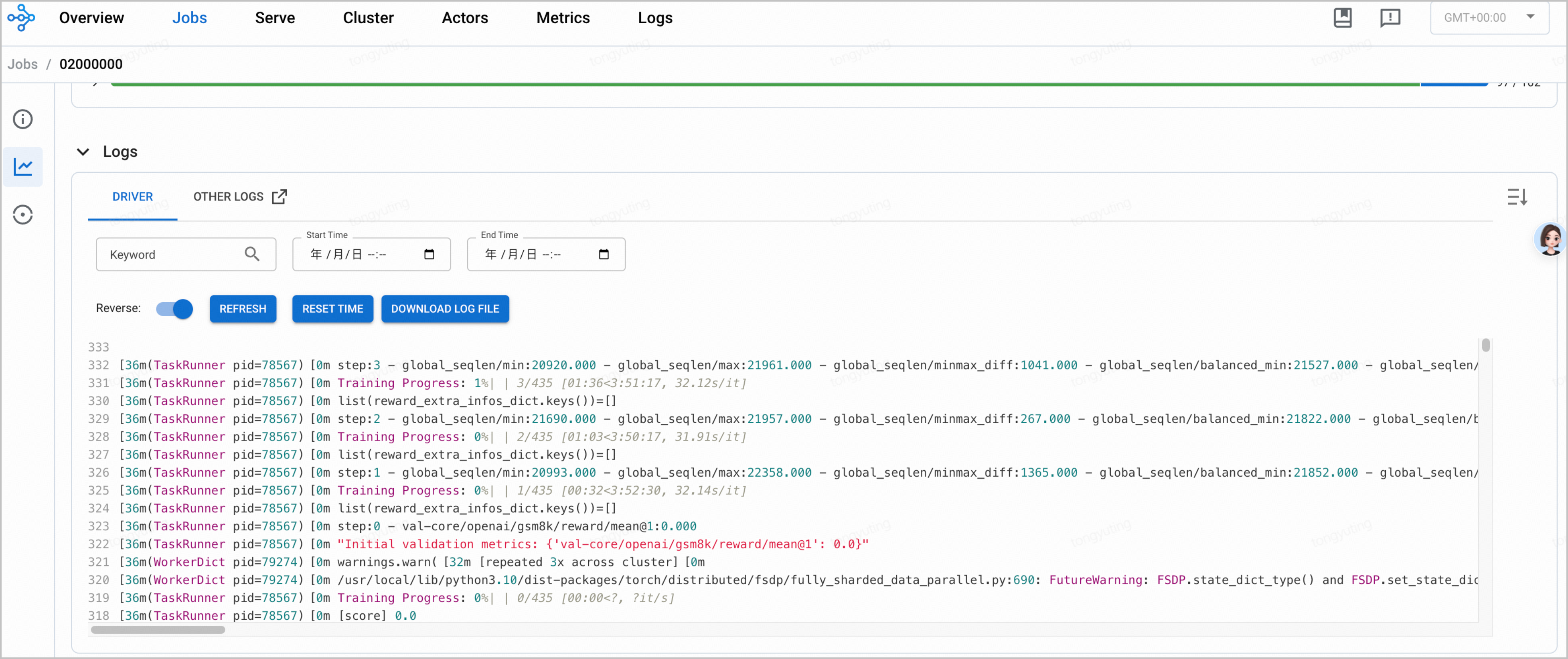
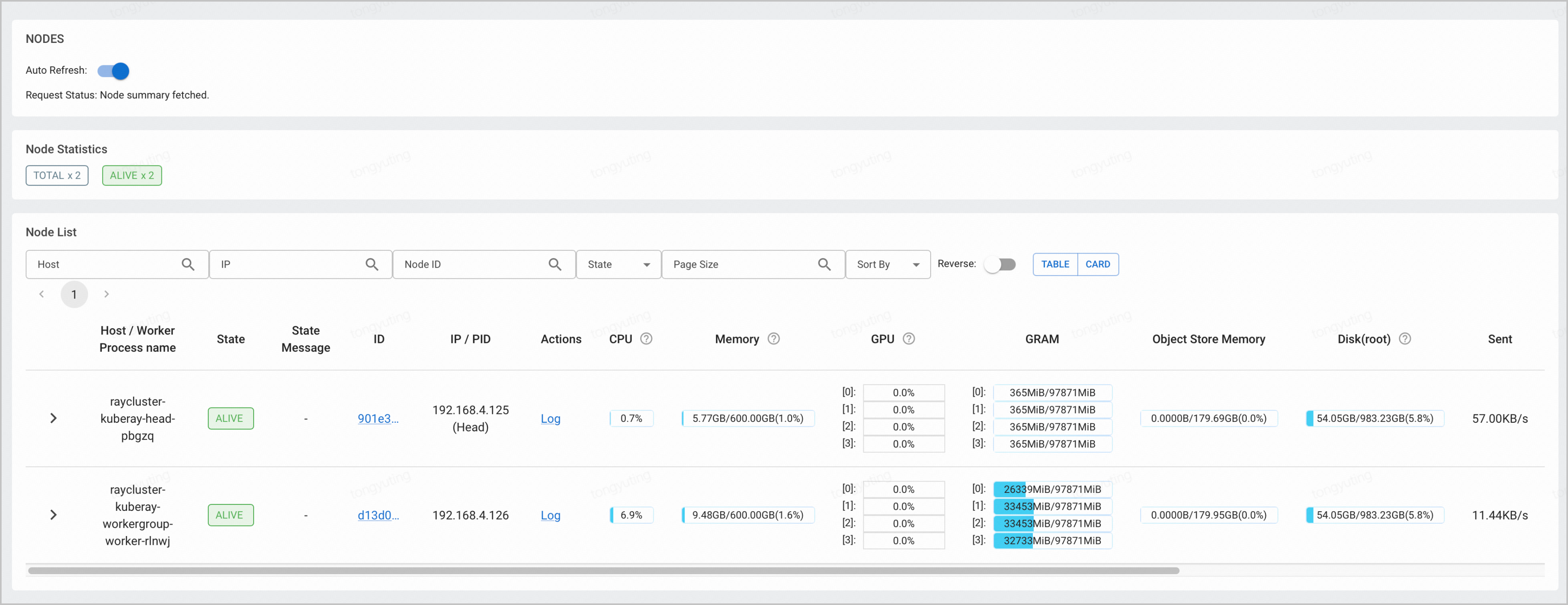
- 创建完成后,在浏览器地址栏直接输入路由规则的 VIP 即可进入 dashboard,可查看训练任务日志和集群状态。
-

-

-
-
开启观测配置
基础观测
开启观测配置
- 登录 容器服务控制台。
- 在顶部导航栏,选择您业务所在地域。
- 在左侧导航栏单击 集群,找到目标集群,单击集群名称。
- 在集群管理页面的左侧导航栏中,选择 云原生观测 > 概览,进入服务开通页面。
- 按照页面指引开启云原生观测和容器监控。
-
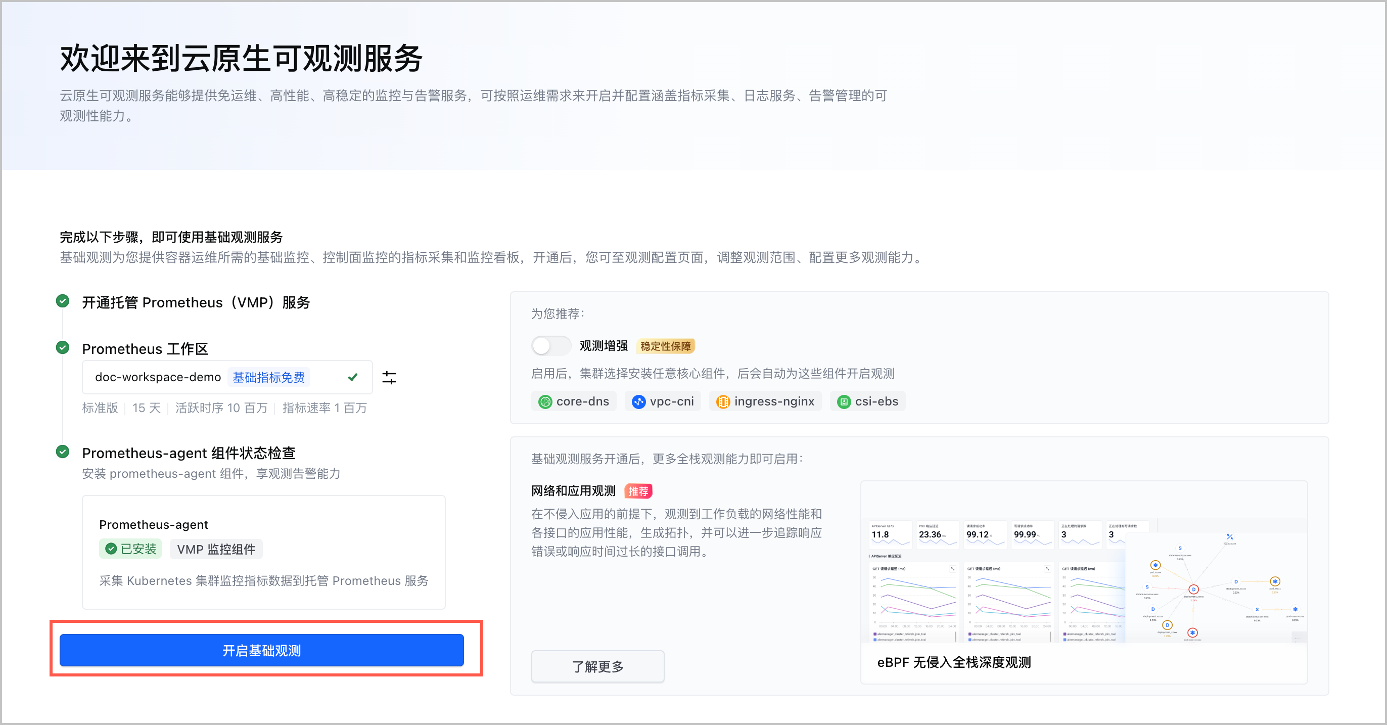
说明
- 创建采集配置,采集 Ray head node 和 worker node 的指标。
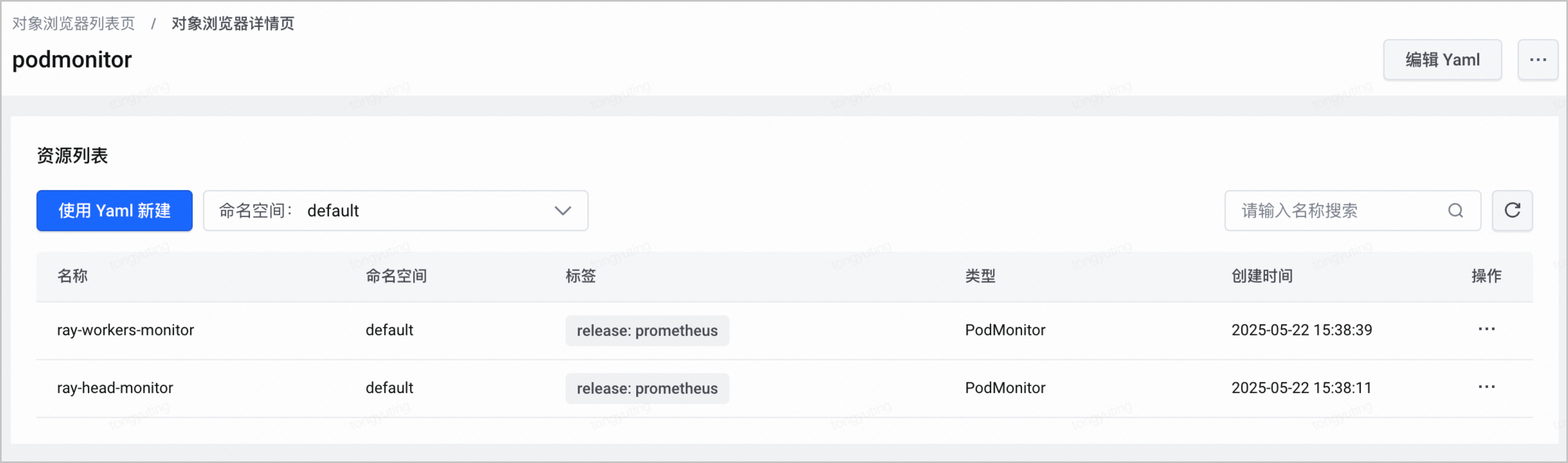
- 首先请确认集群里是否已经存在 ray 的 PodMonitor,如果没有则需要创建。
- 确认方式:在集群管理页面左侧菜单栏中选 工作负载 > 对象浏览器。搜索 PodMonitor,单击进入详情页后,搜索是否有 ray 相关的采集配置。如下图所示。
-
- 如果已经创建了 PodMonitor,请确认 PodMonitor 资源上 存在 标签volcengine.vmp: "true"。如果没有该标签,不会被 Prometheus-agent 识别到,无法采集监控指标。
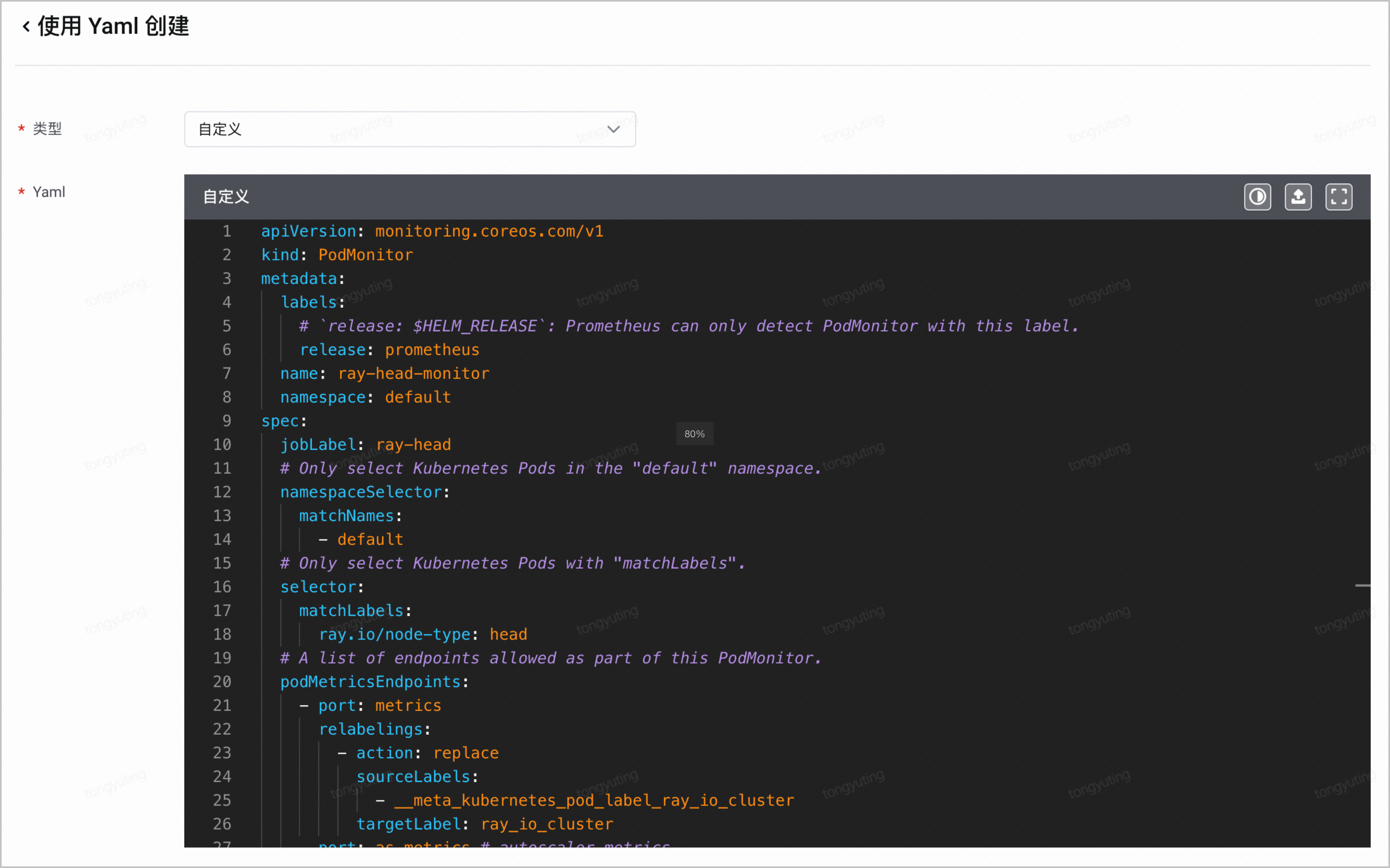
- 在集群管理页面的左侧导航栏中,选择 工作负载 > 对象浏览器,单击 使用 Yaml 创建, 类型 选择 自定义,创建采集配置。
- Head node 的采集配置 PodMonitor。
apiVersion: monitoring.coreos.com/v1
kind: PodMonitor
metadata:
labels:
volcengine.vmp: "true"
name: ray-head-monitor
namespace: default
spec:
jobLabel: ray-head
# Only select Kubernetes Pods in the "default" namespace.
namespaceSelector:
matchNames:
- default
# Only select Kubernetes Pods with "matchLabels".
selector:
matchLabels:
ray.io/node-type: head
# A list of endpoints allowed as part of this PodMonitor.
podMetricsEndpoints:
- port: metrics
relabelings:
- action: replace
sourceLabels:
- __meta_kubernetes_pod_label_ray_io_cluster
targetLabel: ray_io_cluster
- port: as-metrics # autoscaler metrics
relabelings:
- action: replace
sourceLabels:
- __meta_kubernetes_pod_label_ray_io_cluster
targetLabel: ray_io_cluster
- port: dash-metrics # dashboard metrics
relabelings:
- action: replace
sourceLabels:
- __meta_kubernetes_pod_label_ray_io_cluster
targetLabel: ray_io_cluster
- Worker Node 的采集配置 PodMonitor。
apiVersion: monitoring.coreos.com/v1
kind: PodMonitor
metadata:
name: ray-workers-monitor
namespace: default
labels:
volcengine.vmp: "true"
spec:
jobLabel: ray-workers
# Only select Kubernetes Pods in the "default" namespace.
namespaceSelector:
matchNames:
- default
# Only select Kubernetes Pods with "matchLabels".
selector:
matchLabels:
ray.io/node-type: worker
# A list of endpoints allowed as part of this PodMonitor.
podMetricsEndpoints:
- port: metrics
relabelings:
- sourceLabels: [__meta_kubernetes_pod_label_ray_io_cluster]
targetLabel: ray_io_cluster
说明
请关注和修改以下部分:
- namespace:PodMonitor 所在的命名空间,理论上可创建在任意命名空间。
- namespaceSelector:选择匹配哪些命名空间下的 Pod,请修改成 ray 所在的命名空间。
查看监控面板
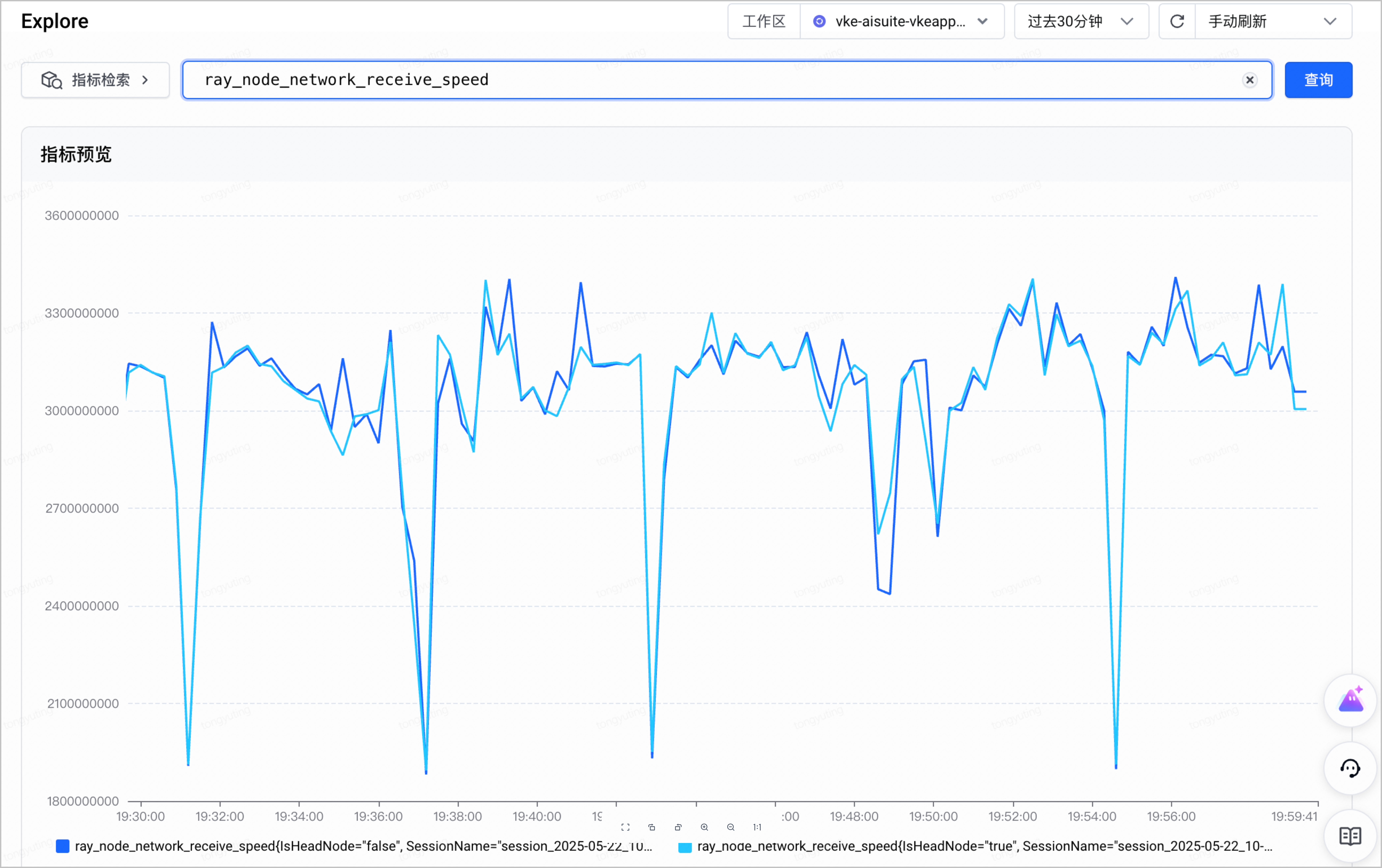
采集规则配置完成后,集群中 ray 的相关指标就被采集并保持在托管 Prometheus 工作区中,您可以使用托管 Prometheus 查看指标或大盘。
- 登录 VMP 服务控制台。
- 在顶部导航栏,选择目标地域。
- 单击左侧导航栏的 Explore,进入 Explore 页面,查询指标。
-
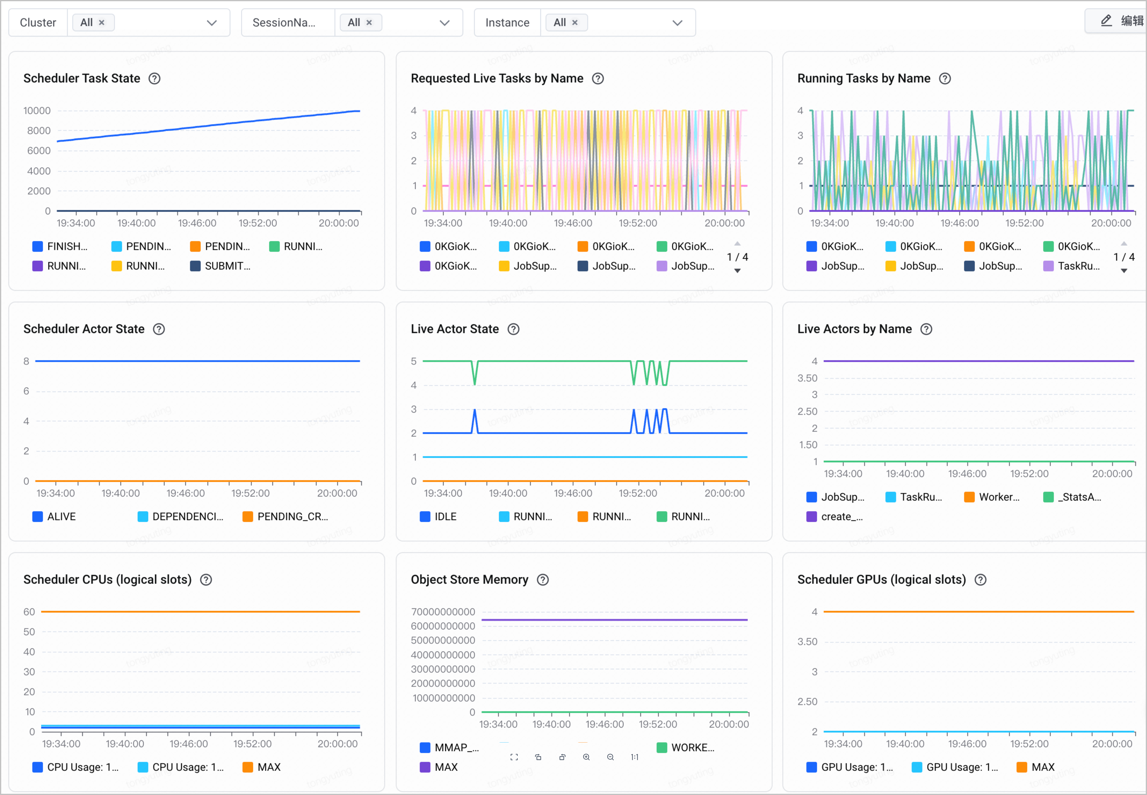
- 单击左侧导航栏的 监控看板,进入监控看板页面。搜索 ray,即可查看 ray 相关看板。
说明
- ray 看板为邀测功能,如需查看,请联系您的客户经理。
- (可选)使用 Grafana 查看 ray 监控。
- 如果希望使用 Grafana 查看 ray 的监控图表,您也可以在 VKE 集群中自行部署 Grafana。
- 搭建 grafana 服务。详情请参见 在容器服务集群中部署 Grafana 并接入工作区。
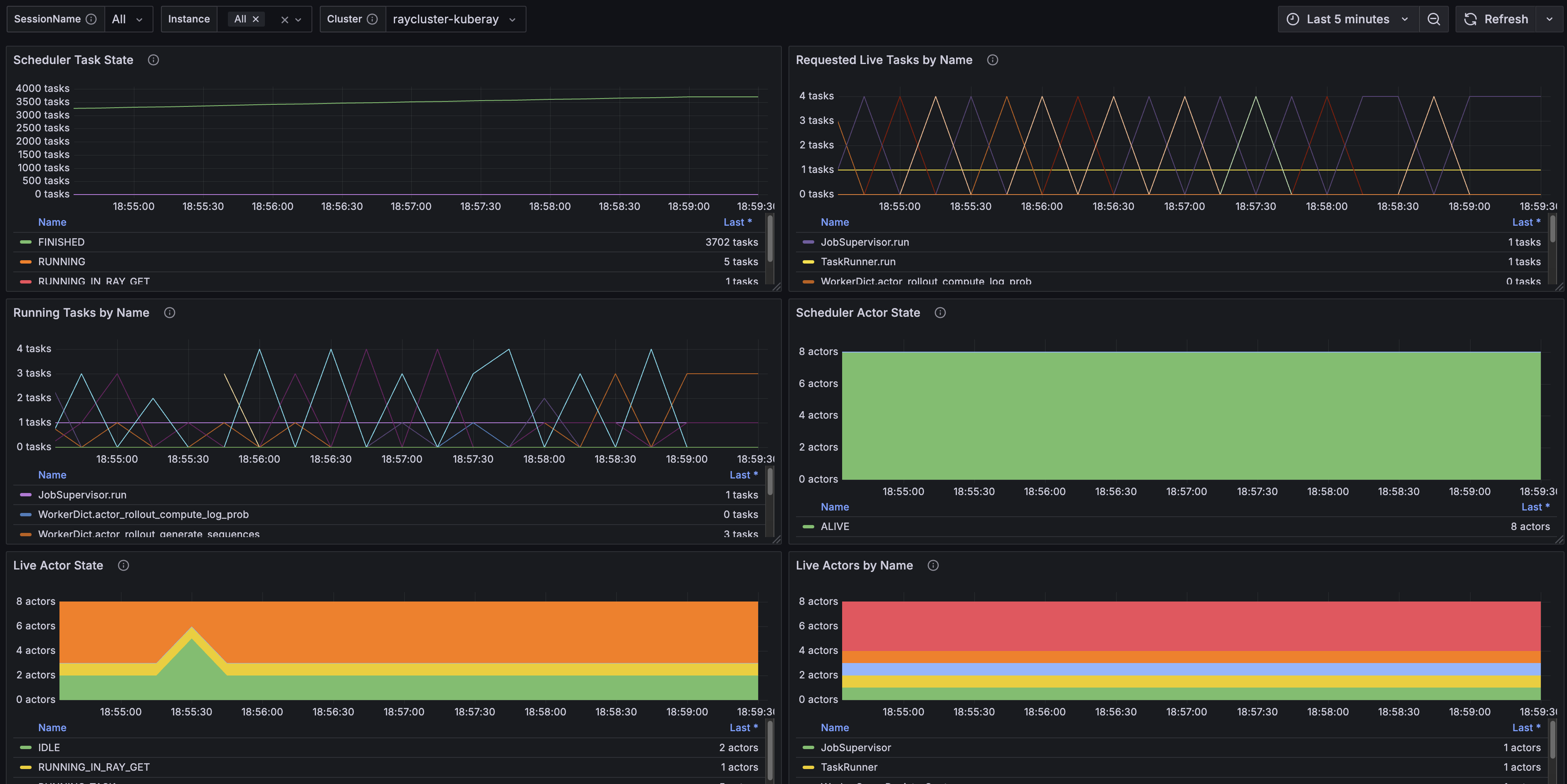
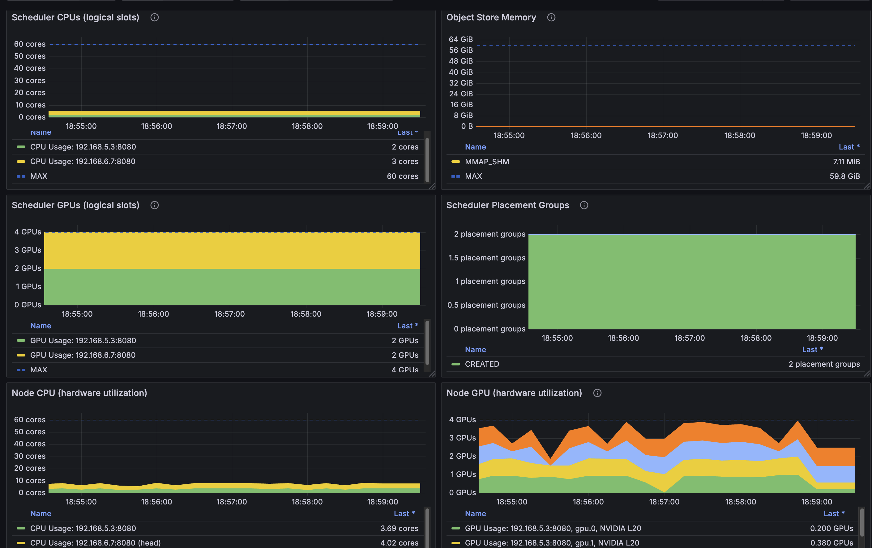
- 登录自建 grafana ,选择导入看版。导入以下看板,导入数据源选 VMP。
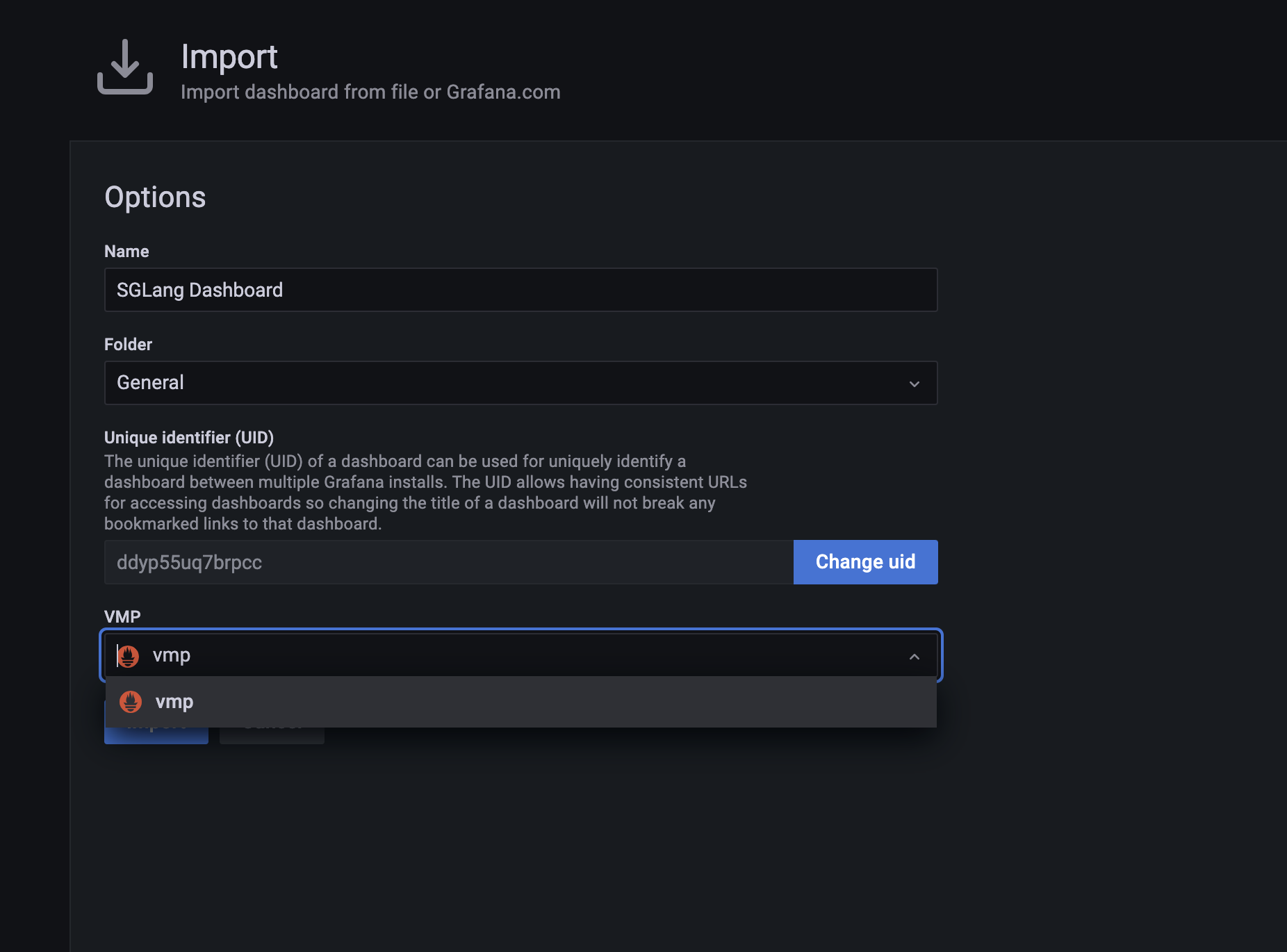
导入后效果如图所示。
深度观测
开启观测配置
- 部署 APMPlus 观测组件。在 VKE 集群控制台左侧导航栏中选择 组件管理,并选择 监控 页签,找到 apmplus-opentelemetry-collector 和 apmplus-server-agent 两个组件并进行安装。安装完成后如下图所示,确认两个组件都是已安装状态且无异常提示。
-

- 给 ray 相关实例增加以下注解,开启添加深度观测。
key | value |
instrumentation.apmplus.volcengine.com/inject-python | true |
在 RayCluster 部署 Yaml 中,添加以下修改。
apiVersion: ray.io/v1
kind: RayCluster
metadata:
creationTimestamp: "2025-05-23T05:23:37Z"
generation: 2
name: raycluster-kuberay
namespace: default
resourceVersion: "52584"
uid: cdb81f16-e53d-481f-9426-5db7f93155b5
spec:
headGroupSpec:
rayStartParams:
dashboard-host: 0.0.0.0
tracing-startup-hook: ray.util.tracing.setup_local_tmp_tracing:setup_tracing
serviceType: ClusterIP
template:
metadata:
annotations:
instrumentation.apmplus.volcengine.com/inject-python: "true"
spec:
containers:
- env:
- name: OTEL_PYTHON_DISABLED_INSTRUMENTATIONS
value: system_metrics
- image: cr-helm-test-cn-beijing.cr.volces.com/cr-helm-test/verl:ngc-th2.6.0-cu126-vllm0.8.4-flashinfer0.2.2-cxx11abi0-custom-v1
imagePullPolicy: IfNotPresent
name: ray-head
resources:
limits:
cpu: "60"
memory: 600Gi
nvidia.com/gpu: 4
requests:
cpu: "60"
memory: 600Gi
nvidia.com/gpu: 4
volumeMounts:
- mountPath: /tmp/ray
name: log-volume
- mountPath: /data
name: tos-pv
volumes:
- emptyDir: {}
name: log-volume
- name: tos-pv
persistentVolumeClaim:
claimName: verl-pvc
workerGroupSpecs:
- groupName: workergroup
maxReplicas: 3
minReplicas: 1
numOfHosts: 1
rayStartParams: {}
replicas: 1
template:
metadata:
annotations:
instrumentation.apmplus.volcengine.com/inject-python: "true"
spec:
containers:
- env:
- name: OTEL_PYTHON_DISABLED_INSTRUMENTATIONS
value: system_metrics
- image: cr-helm-test-cn-beijing.cr.volces.com/cr-helm-test/verl:ngc-th2.6.0-cu126-vllm0.8.4-flashinfer0.2.2-cxx11abi0-custom-v1
imagePullPolicy: IfNotPresent
name: ray-worker
resources:
limits:
cpu: "60"
memory: 600Gi
nvidia.com/gpu: 4
requests:
cpu: "60"
memory: 600Gi
nvidia.com/gpu: 4
volumeMounts:
- mountPath: /tmp/ray
name: log-volume
- mountPath: /data
name: tos-pv
volumes:
- emptyDir: {}
name: log-volume
- name: tos-pv
persistentVolumeClaim:
claimName: verl-pvc
status:
availableWorkerReplicas: 1
conditions:
- lastTransitionTime: "2025-05-23T07:23:08Z"
message: ""
reason: HeadPodRunningAndReady
status: "True"
type: HeadPodReady
- lastTransitionTime: "2025-05-23T05:29:39Z"
message: All Ray Pods are ready for the first time
reason: AllPodRunningAndReadyFirstTime
status: "True"
type: RayClusterProvisioned
- lastTransitionTime: "2025-05-23T05:23:37Z"
message: ""
reason: RayClusterSuspended
status: "False"
type: RayClusterSuspended
- lastTransitionTime: "2025-05-23T05:23:37Z"
message: ""
reason: RayClusterSuspending
status: "False"
type: RayClusterSuspending
desiredCPU: "60"
desiredGPU: "4"
desiredMemory: 200Gi
desiredTPU: "0"
desiredWorkerReplicas: 1
endpoints:
client: "10001"
dashboard: "8265"
gcs-server: "6379"
metrics: "8080"
serve: "8000"
head:
podIP: 192.168.5.38
podName: raycluster-kuberay-head-wcrb7
serviceIP: 192.168.5.38
serviceName: raycluster-kuberay-head-svc
lastUpdateTime: "2025-05-23T07:23:24Z"
maxWorkerReplicas: 3
minWorkerReplicas: 1
observedGeneration: 2
readyWorkerReplicas: 1
state: ready
stateTransitionTimes:
ready: "2025-05-23T05:29:39Z"
- 设置 ray tracing。
若要启用 tracing 功能,您必须提供一个 tracing 启动脚本,脚本中包含一个用于设置 tracing provider 和 span processor 的函数。该函数无入参且需要保证在所有工作进程的 Python 环境中都可用。
以下是一个示例,会根据环境变量配置把 tracing 数据发送到服务端,当 apmplus-opentelemetry-collector 和 apmplus-server-agent 组件安装完成后,环境变量会被配置为 apmplus-opentelemetry-collector 。该代码已在镜像中自动包含。
import ray
import logging
from opentelemetry import trace
from opentelemetry.sdk.trace import TracerProvider
from opentelemetry.sdk.trace.export import (
BatchSpanProcessor,
)
from opentelemetry.exporter.otlp.proto.http.trace_exporter import (
OTLPSpanExporter as HTTPExporter,
)
def setup_tracing() -> None:
logging.warning("setup_tracing")
trace.set_tracer_provider(TracerProvider())
trace.get_tracer_provider().add_span_processor(
BatchSpanProcessor(
HTTPExporter()
)
)
RayCluster yaml 中 rayStartParams 添加如下参数。
spec:
headGroupSpec:
serviceType: ClusterIP
rayStartParams:
dashboard-host: "0.0.0.0"
tracing-startup-hook: "tracing.setup_tracing:setup_tracing"
template:
查看观测数据
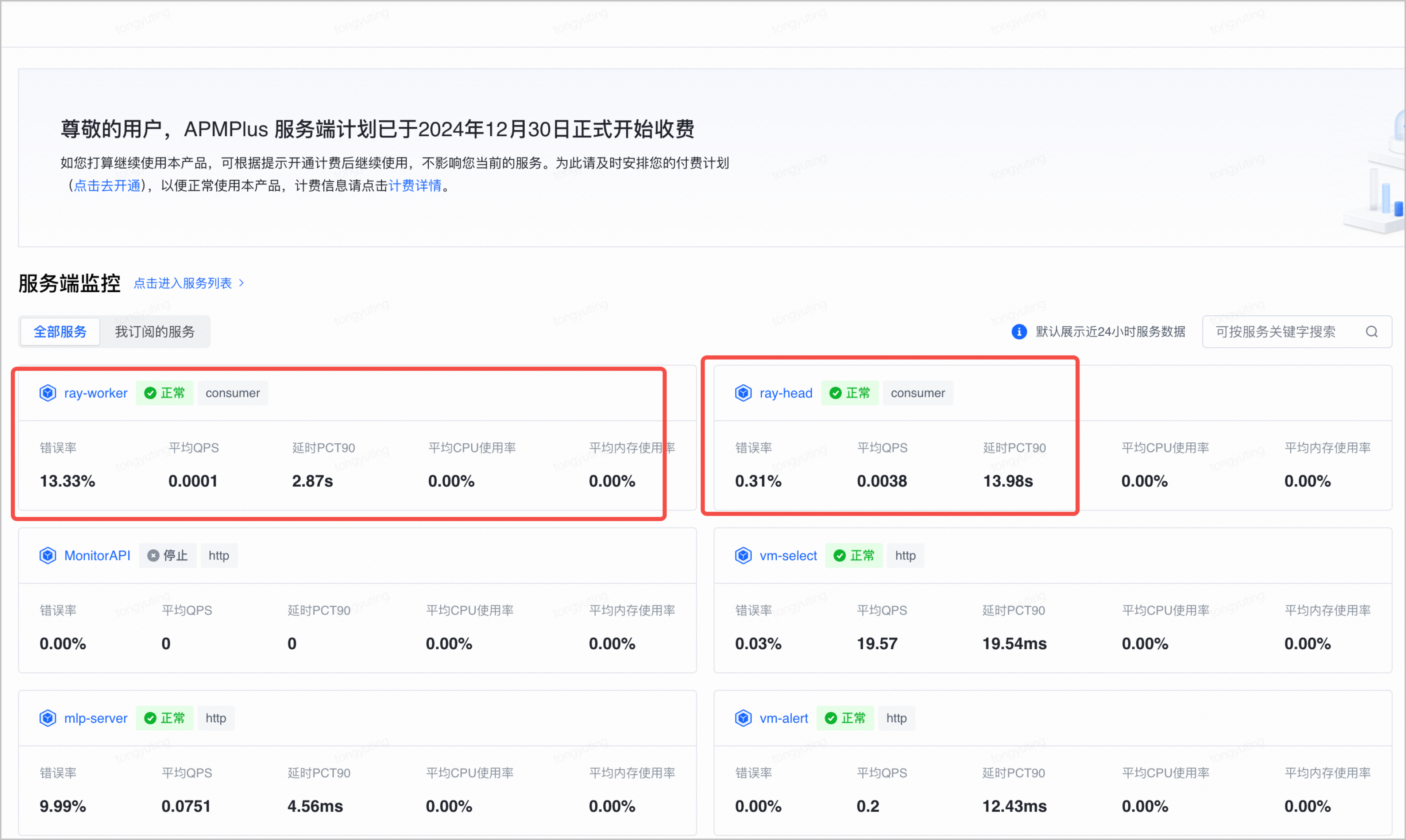
- 开启观测配置后,产生的 tracing 数据会发送到 APMPlus 中,在应用性能监控全链路版云产品服务页面,选择 服务端监控,即可查看 ray-worker 和 ray-header 两个服务。
-
- 单击服务名称,进入观测看板页面。
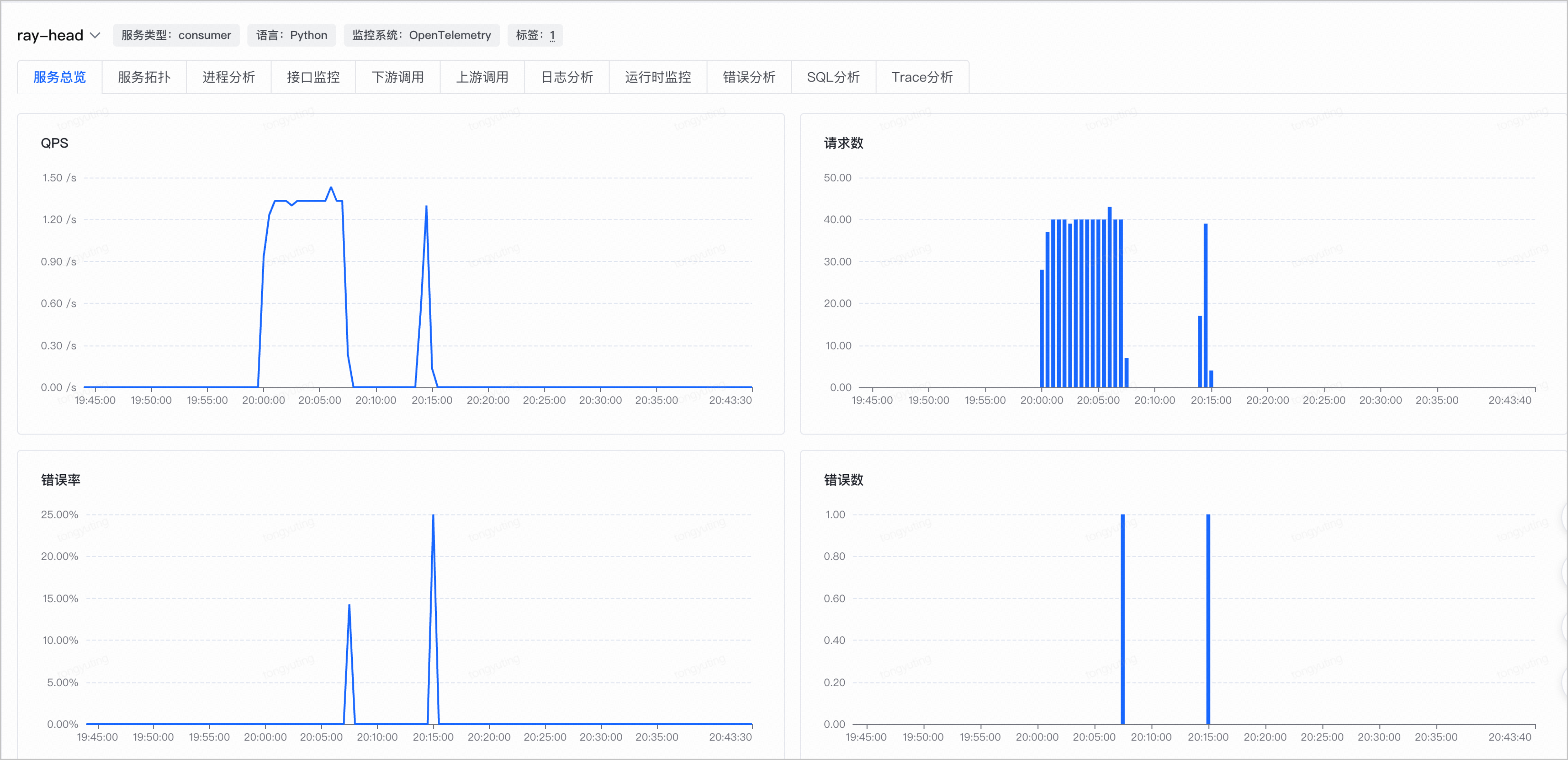
- 在 服务总览 页签,可查看服务黄金指标,例如:QPS、请求错误率等。
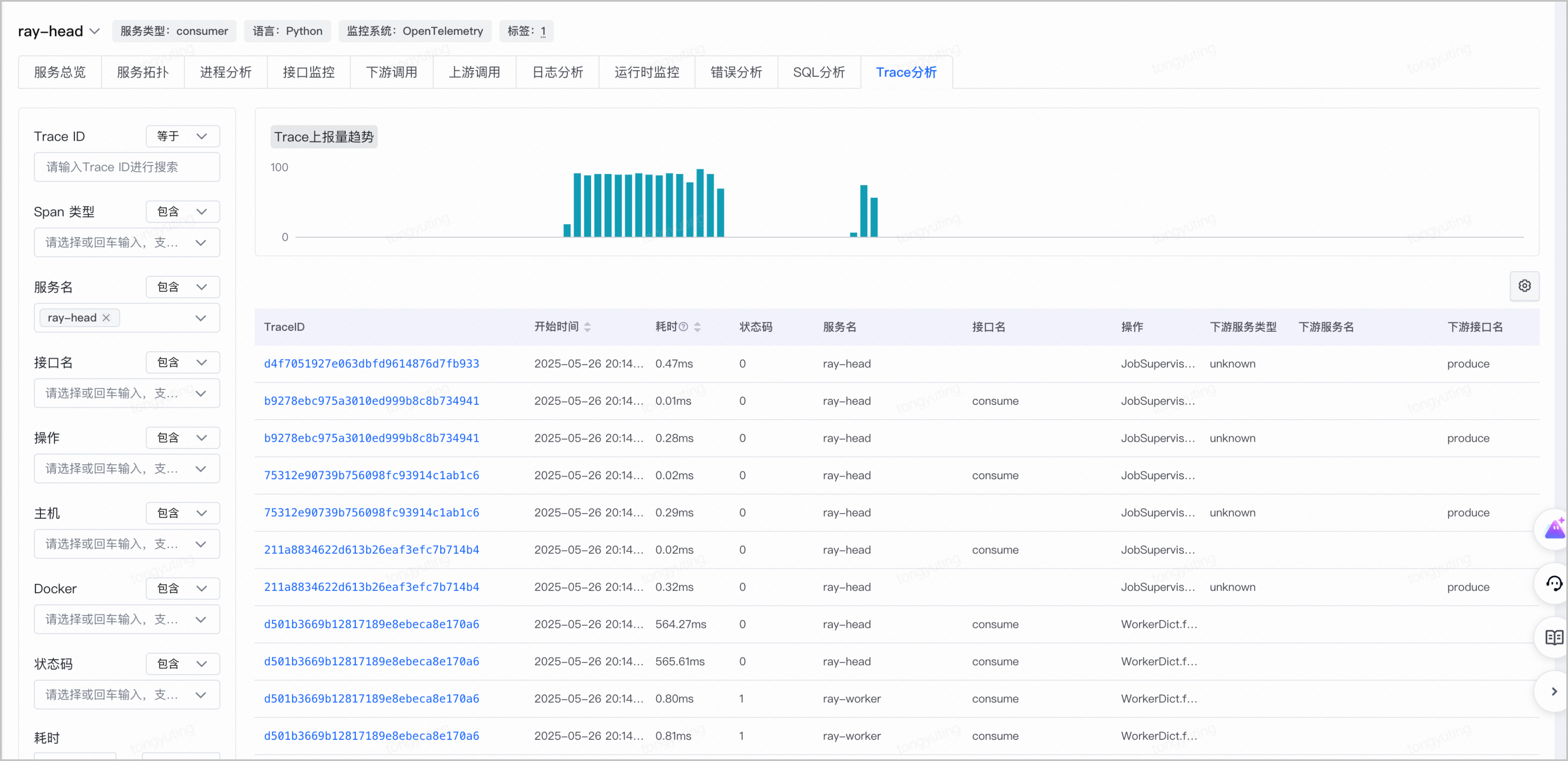
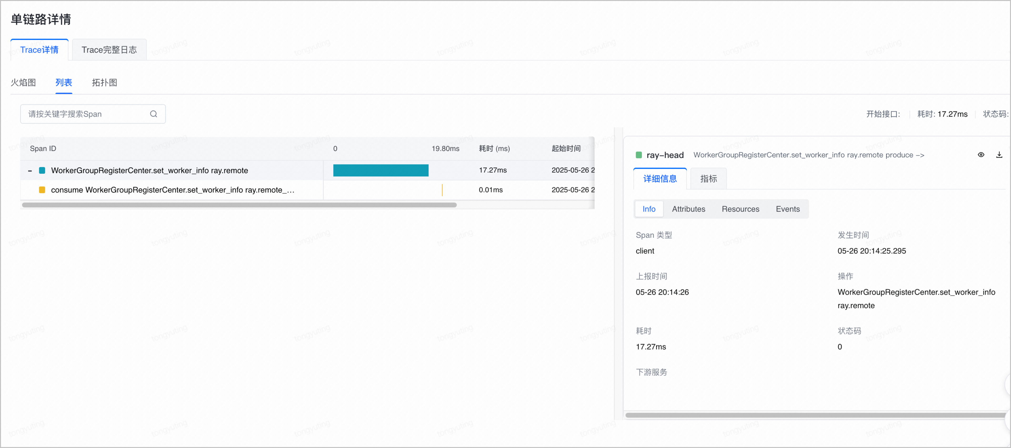
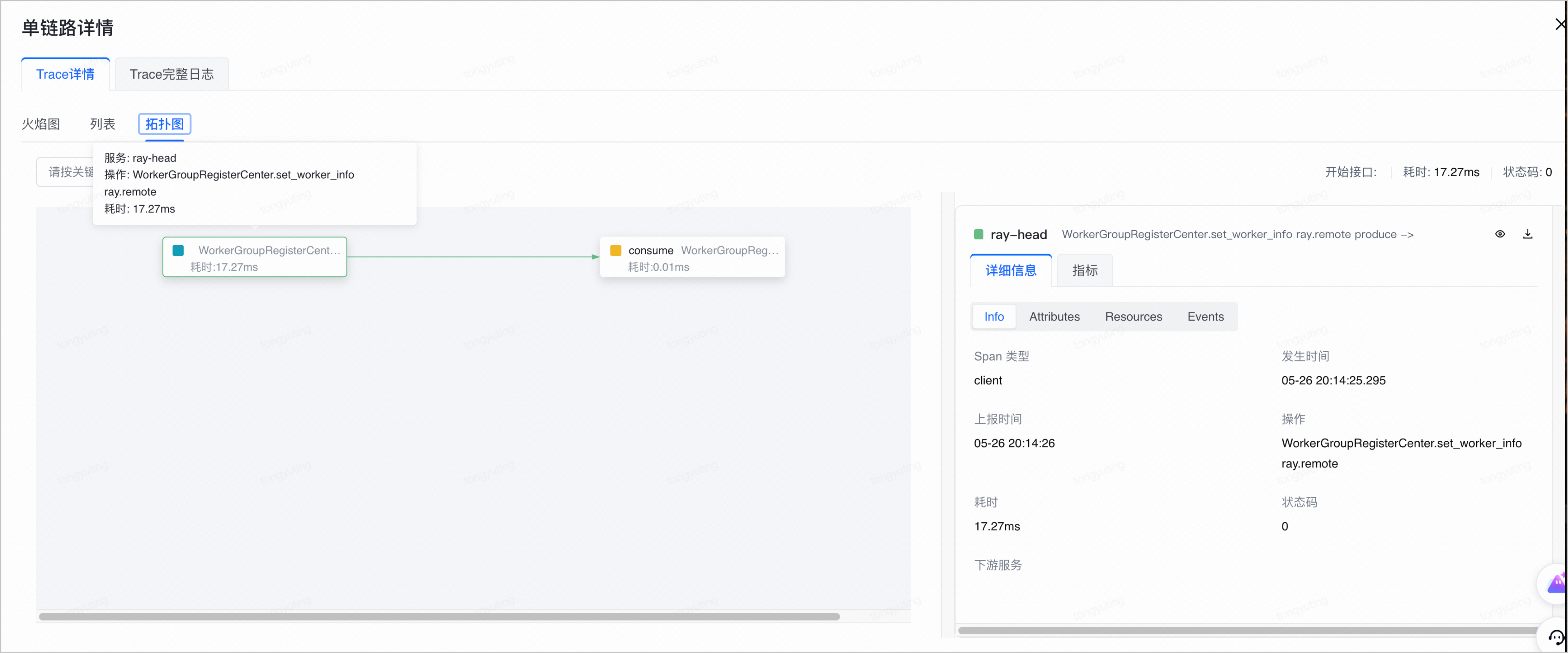
- 在 Trace 分析 页签,可以查看上报的 tracing 链路数据。单击目标 Trace ID,前往单链路详情页面。在列表视图中查看全链路 Trace 信息。
wandb 部署与对接
Weights & Biases(简称 Weights & Biases,缩写为 wandb) 是一个用于机器学习实验跟踪与管理的工具平台,旨在帮助数据科学家和机器学习工程师更高效地开发、优化和部署模型。它提供了一套简洁的工具,可自动记录实验过程中的关键指标、可视化结果、管理代码版本和数据集,并支持团队协作。
本节介绍如何在上述集群中部署本地版 wandb,并将 veRL的训练指标推送到 wandb 中。
准备镜像
- 先拉取镜像到本地电脑,再推送到自己的镜像仓库,操作步骤请参考 基于 Docker 推送和拉取镜像。
创建 NAS 文件存储
- 登录 文件存储 NAS 控制台。
- 在顶部菜单栏,选择需要创建文件系统的地域。
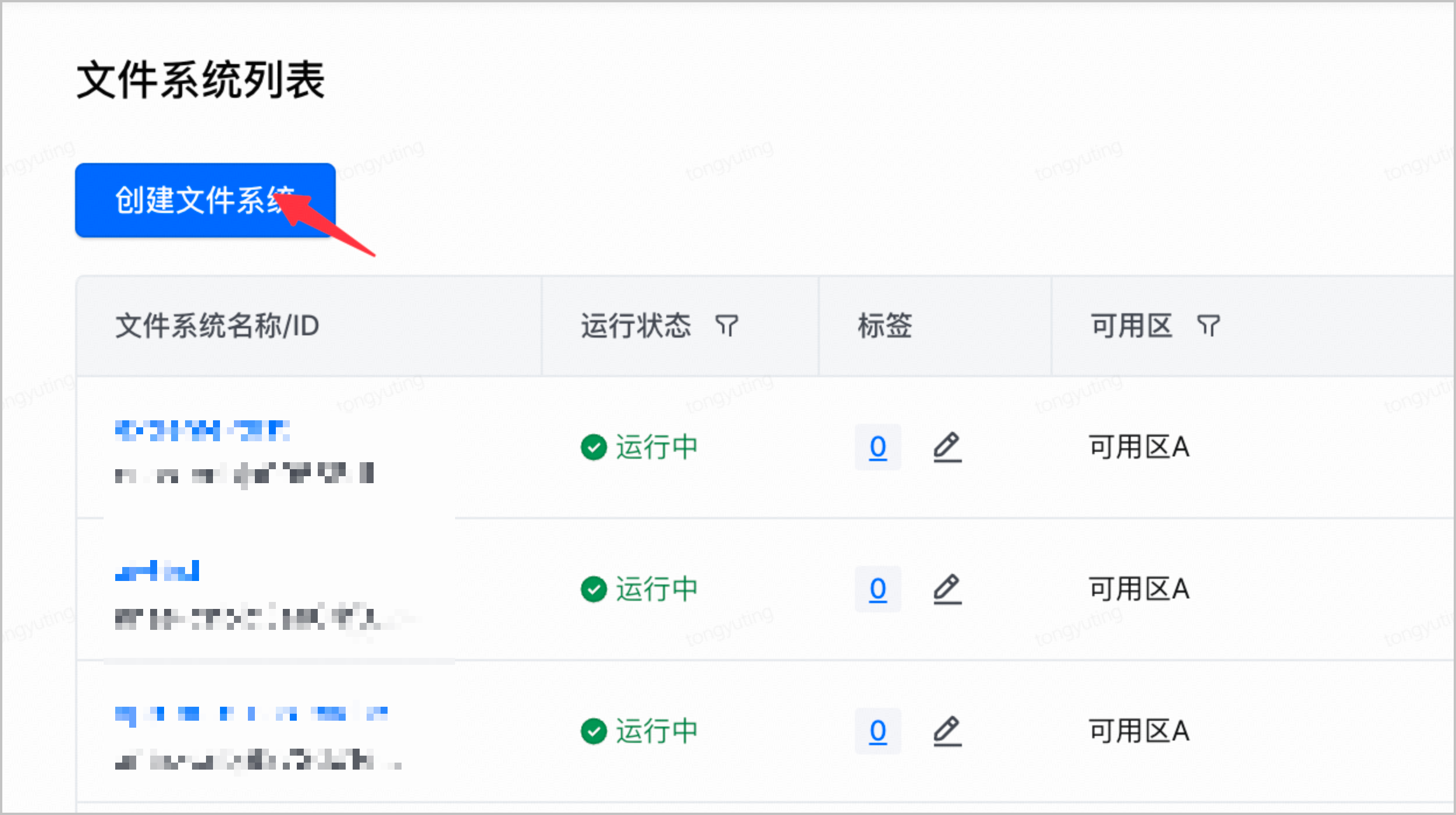
- 在左侧导航栏,选择 文件系统 > 文件系统列表,在 文件系统列表 页面,单击 创建文件系统。
-
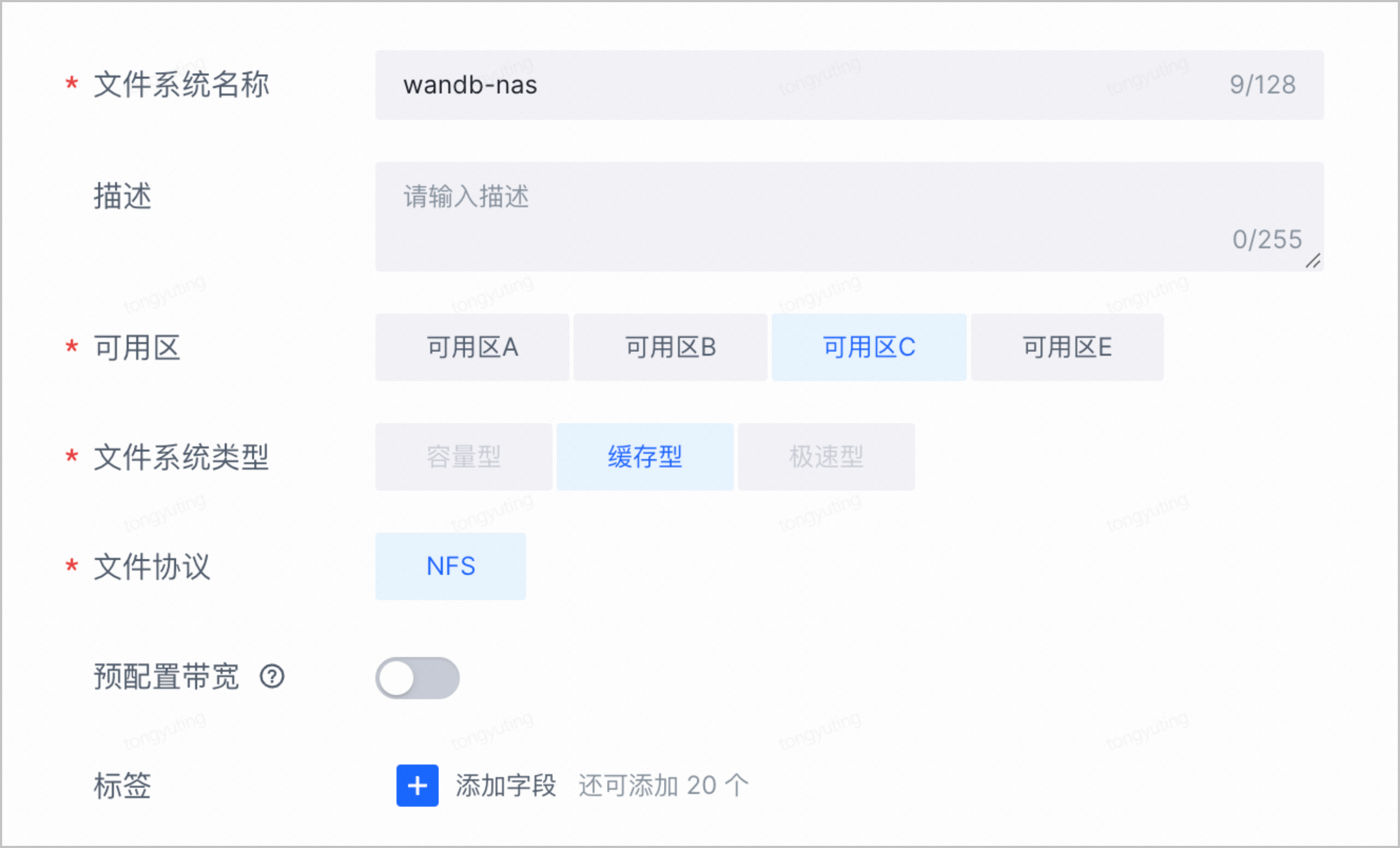
- 配置文件系统,具体参数说明请参考 创建文件系统。
-
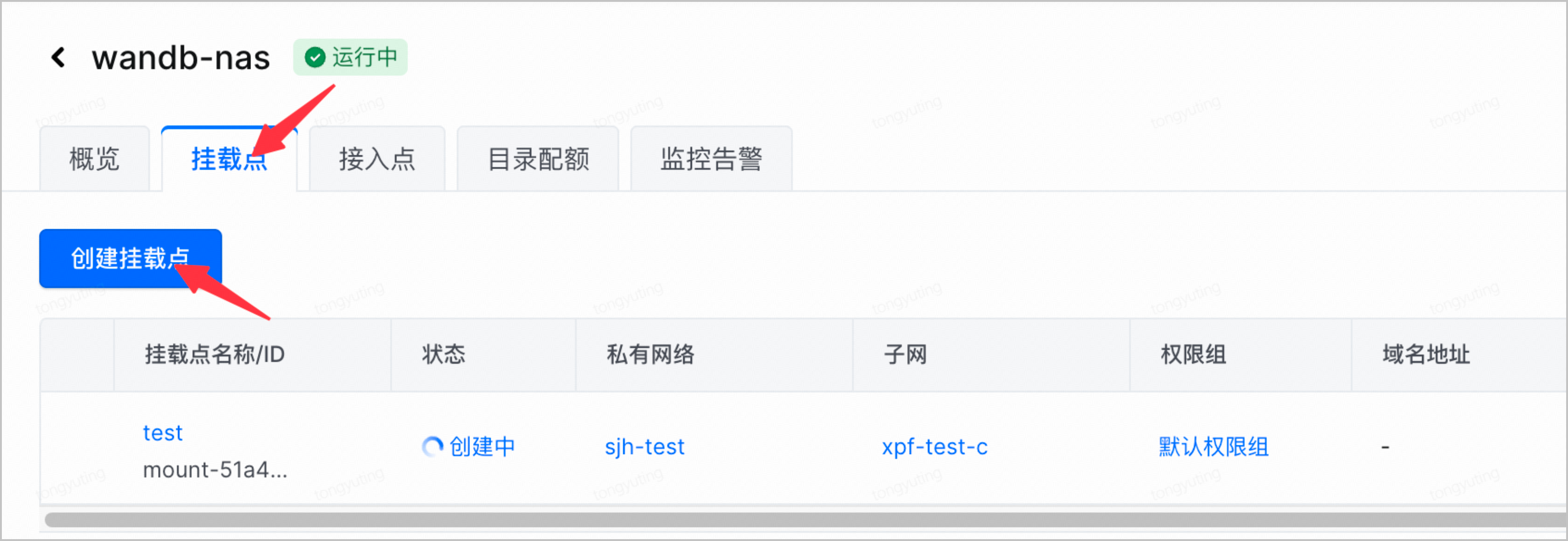
- 单击文件系统名称,进入文件系统详情页,选择 挂载点 页签,单击 创建挂载点。
-
注意
挂载点的私有网络需要选择 VKE 集群所在的 VPC 网络。
- 回到 VKE 集群,创建存储卷(PV),选择刚才已创建的 NAS 和挂载点。
-
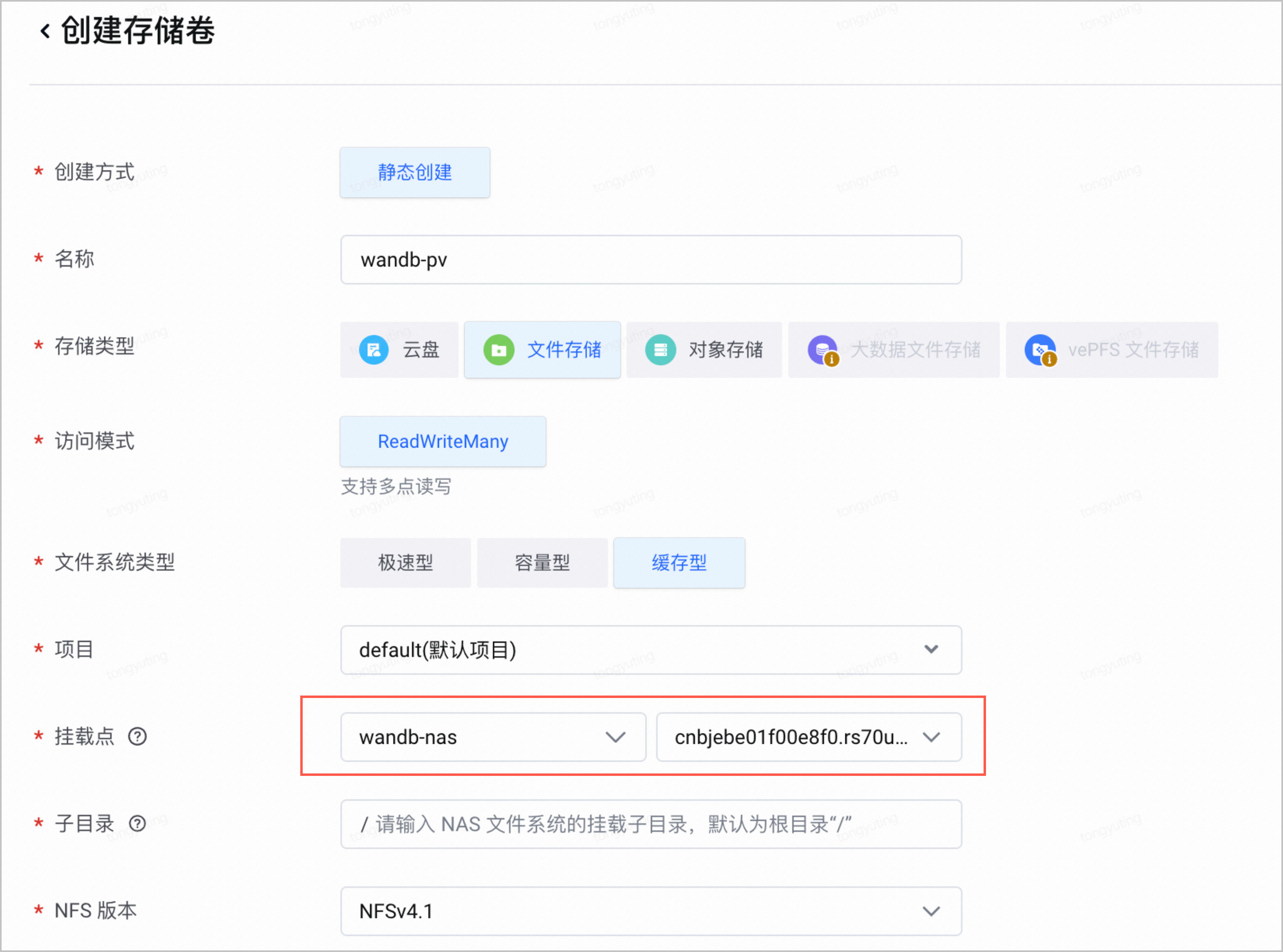
- 创建存储卷声明(PVC),关联创建好的 PV。
-
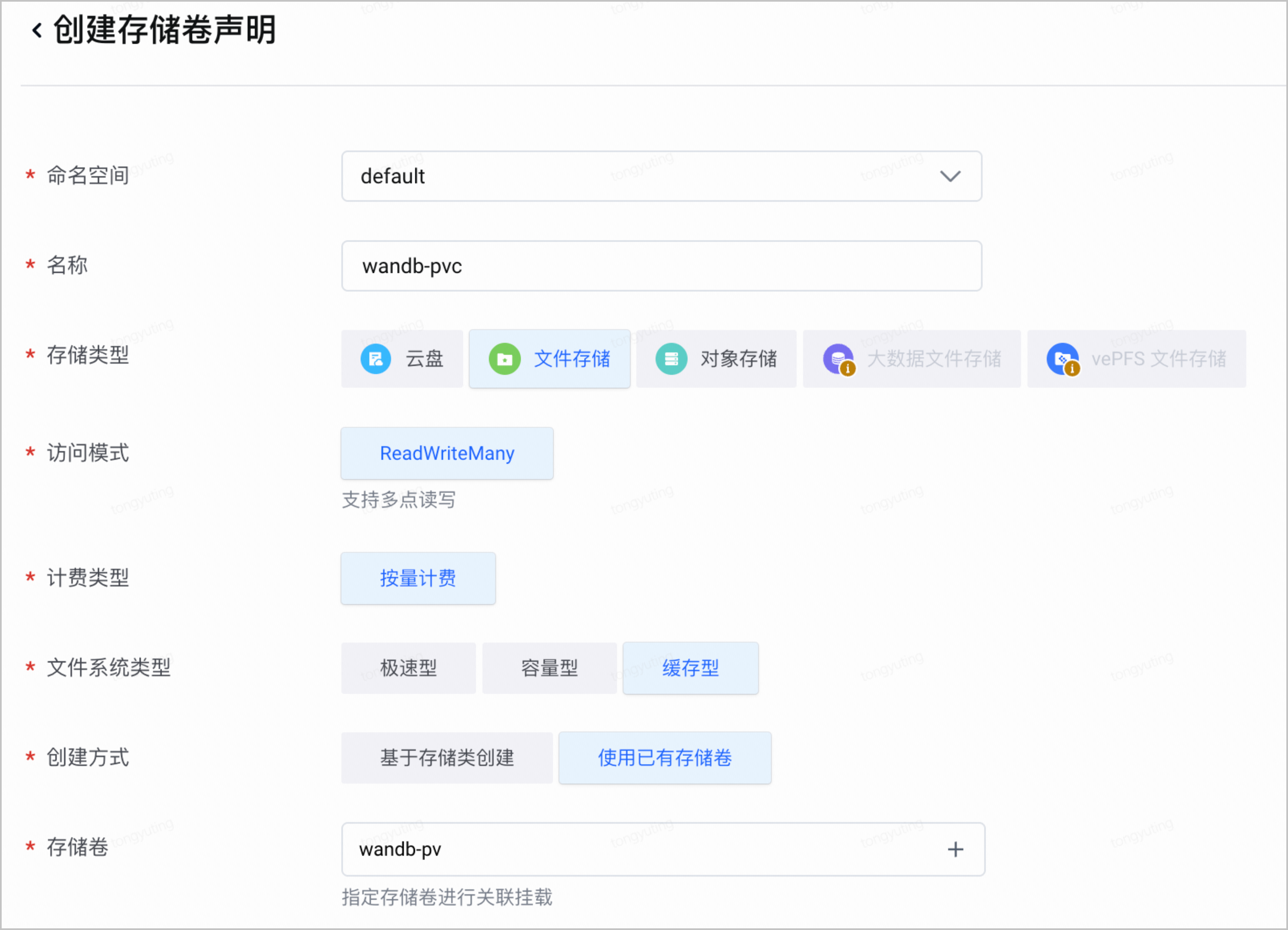
部署 wandb local
- 部署wandb local
- 修改以下 Yaml 内容,根据实际修改 wandb local 镜像地址和 PVC 名称。
apiVersion: apps/v1
kind: Deployment
metadata:
name: wandb
labels:
app: wandb
spec:
strategy:
type: RollingUpdate
replicas: 1
selector:
matchLabels:
app: wandb
template:
metadata:
labels:
app: wandb
spec:
initContainers:
- name: init-permissions
image: cr-helm-test-cn-beijing.cr.volces.com/cr-helm-test/wandb-local:0.68.2
command: ["sh", "-c", "chmod 777 /vol"]
securityContext:
runAsUser: 0
volumeMounts:
- name: wandb-pv
mountPath: /vol
containers:
- name: wandb
imagePullPolicy: IfNotPresent
image: cr-helm-test-cn-beijing.cr.volces.com/cr-helm-test/wandb-local:0.68.2
ports:
- name: http
containerPort: 8080
protocol: TCP
volumeMounts:
- name: wandb-pv
mountPath: /vol
livenessProbe:
httpGet:
path: /healthz
port: http
readinessProbe:
httpGet:
path: /ready
port: http
resources:
requests:
cpu: "2000m"
memory: 4G
limits:
cpu: "4000m"
memory: 8G
volumes:
- name: wandb-pv
persistentVolumeClaim:
claimName: wandb-pvc
apiVersion: v1
kind: Service
metadata:
name: wandb-service
spec:
type: ClusterIP
selector:
app: wandb
ports:
- protocol: TCP
port: 8080
targetPort: 8080
- 登录 容器服控制台,单击目标集群名称,进入集群管理页面。
- 在左侧导航栏,选择 工作负载 > 对象浏览器。
- 单击 使用 Yaml 创建,选择 类型 为 自定义,填入修改后 Yaml 后,单击右下角 确定 提交,默认部署到 default 命名空间。
- 创建路由规则,对外暴露 wandb 服务。
- 在左侧导航栏,选择 服务与路由 > 路由规则,单击 创建路由规则。
- 需要注意以下列举的参数配置。其余参数说明和详细的操作步骤,请参见 通过控制台创建 ALB Ingress。
- 配置项说明Ingress类型选择 应用型负载均衡ALB。协议选择 HTTP。路径输入 /。服务选择wandb-service:8080。
- 创建完成后,在浏览器地址栏直接输入路由规则的 VIP,即可进入 wandb 管理页面。
-

-

wandb 配置
- 进入 wandb 管理页面,创建账号。(未来需要使用email和密码登录,务必牢记)。
-
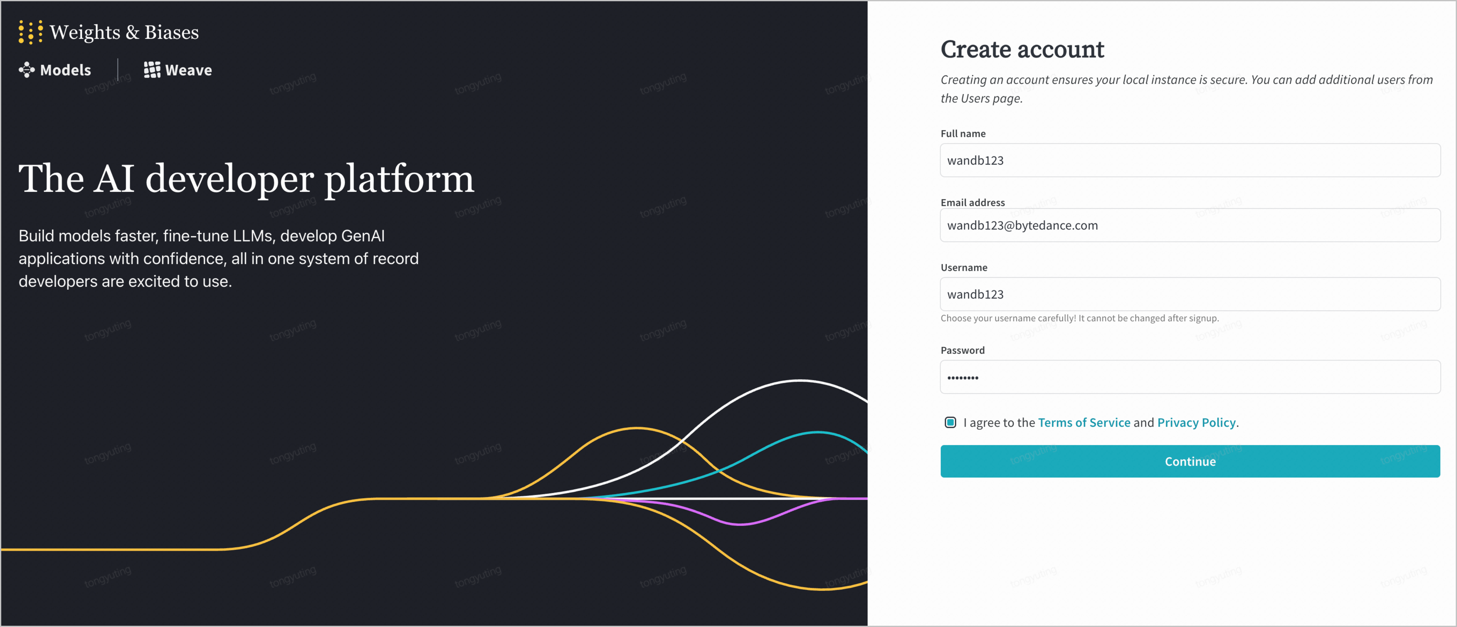
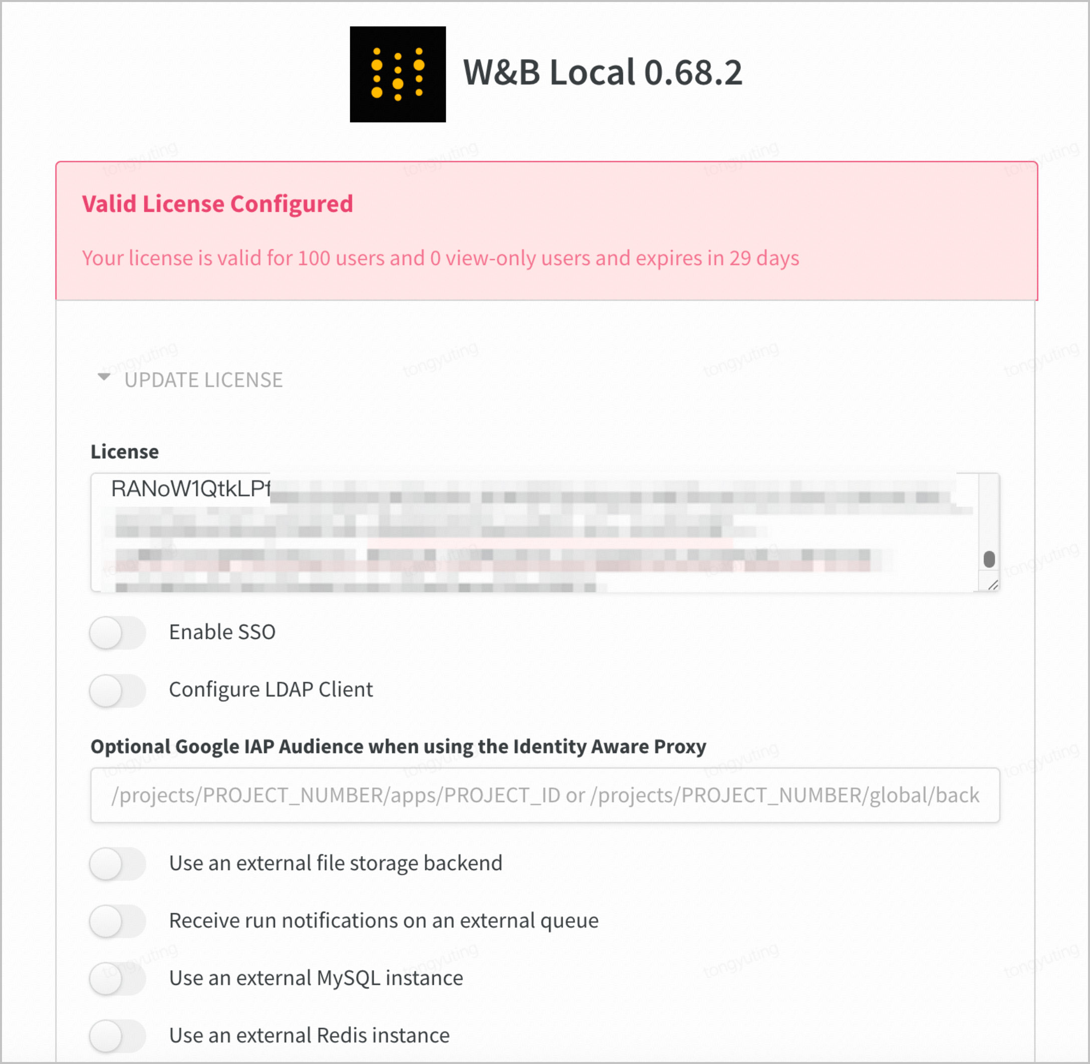
- 配置 license(若无,可按提示申请免费license)。
-
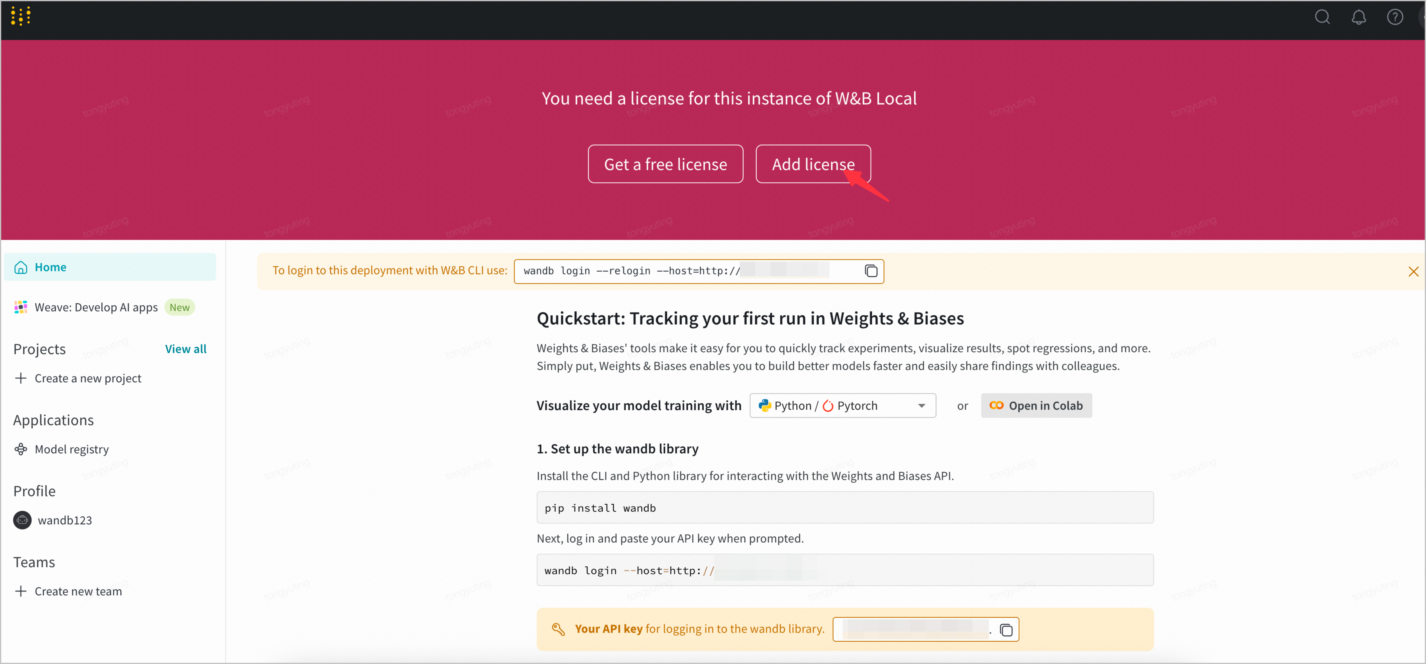
-
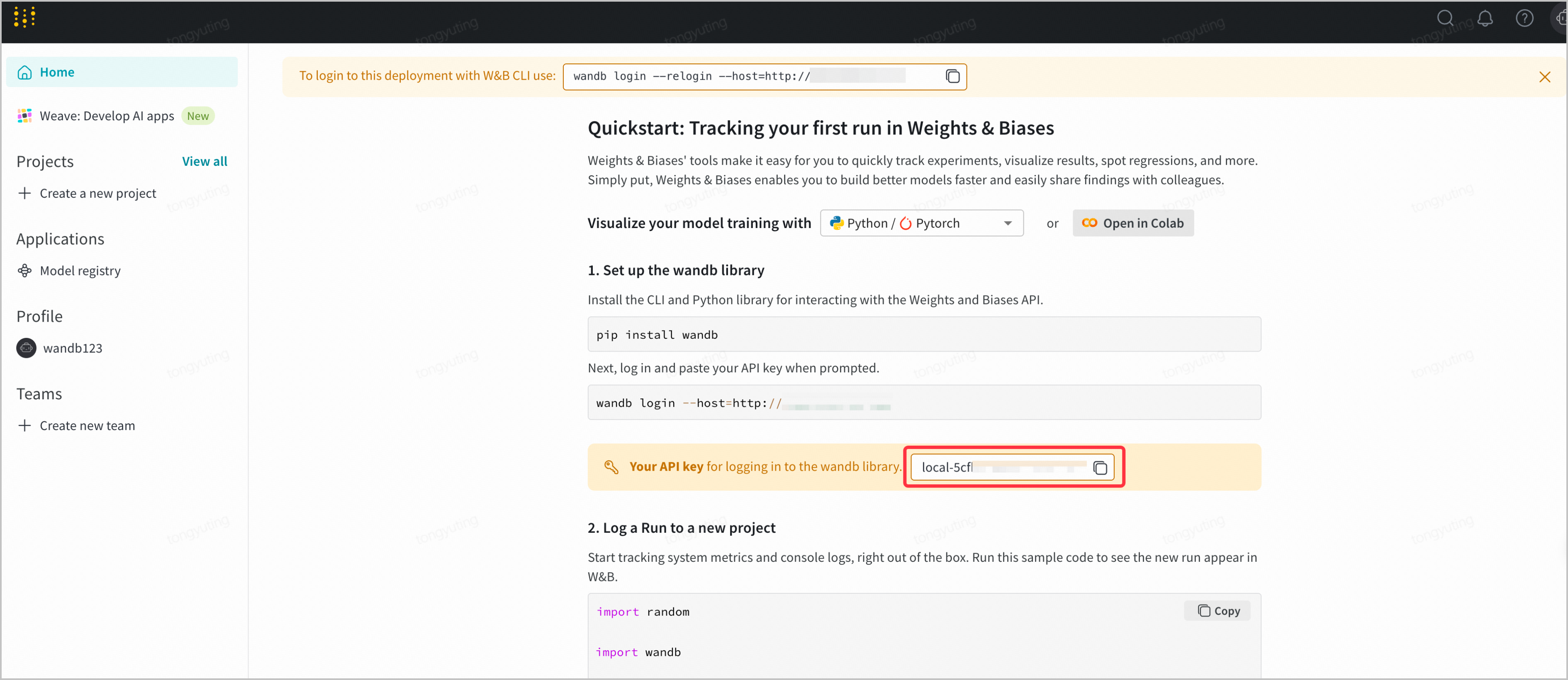
- 回到 Home 页面,查看API Key。
-
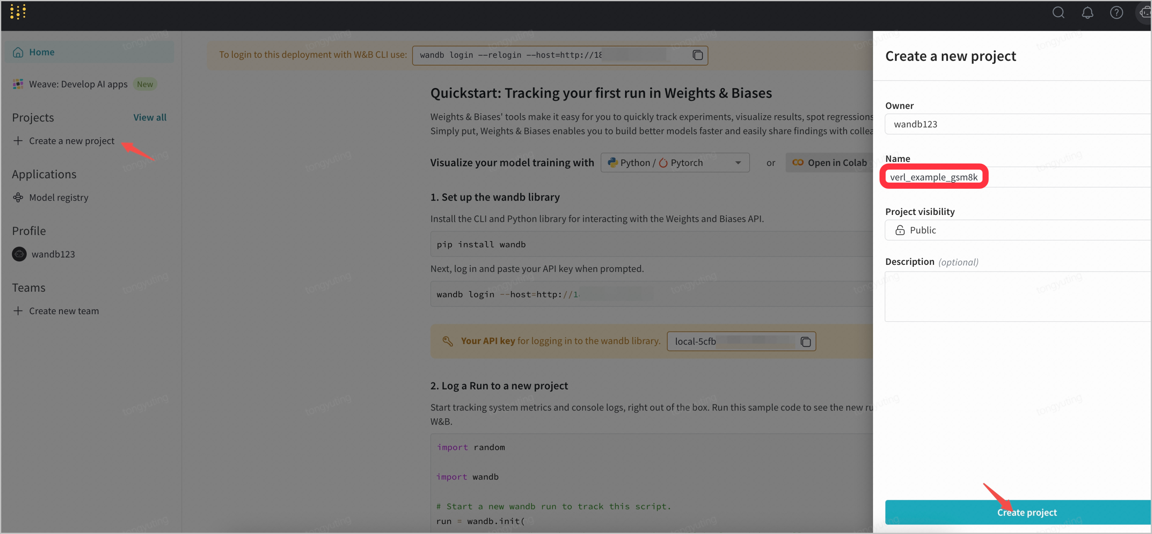
- 创建一个 project。
-
verl 配置
- 参考 提交训练任务 进入 head 容器组控制台,在提交训练任务前,编辑verl/trainer/runtime_env.yaml文件内容,添加以下两行,其中WANDB_API_KEY填写为 API KEY。
working_dir: ./
excludes: ["/.git/"]
env_vars:
TORCH_NCCL_AVOID_RECORD_STREAMS: "1"
# If you are using vllm<=0.6.3, you might need to set the following environment variable to avoid bugs:
# VLLM_ATTENTION_BACKEND: "XFORMERS"
WANDB_BASE_URL: "http://wandb-service:8080"
WANDB_API_KEY: "local-xxxxxxxxxxxxxxxxxxxxxxxxxxxxxxxxxxx"
- 在 VKE 本地提交训练任务命令,添加或修改以下内容,提交训练任务:
- trainer.logger添加'wandb'。
- trainer.project_name填写之前 wandb 中创建好的 project name。
- trainer.experiment_name填写一个实验名称。
- 请将trainer.default_local_dir设置为/data目录内的任意文件夹,即可将训练 checkpoints 保存指定路径。
cd /workspace/verl
ray job submit --address="http://127.0.0.1:8265" \
--runtime-env=verl/trainer/runtime_env.yaml \
--no-wait \
-- \
python3 -m verl.trainer.main_ppo \
algorithm.adv_estimator=gae \
data.train_files=/data/models/Eurus-2-RL-Data/train1000.parquet \
data.val_files=/data/models/Eurus-2-RL-Data/validation.parquet \
data.train_batch_size=128 \
data.max_prompt_length=512 \
data.max_response_length=512 \
data.filter_overlong_prompts=True \
data.truncation='error' \
actor_rollout_ref.model.path=/data/models/Qwen2.5-7B-Instruct-1M \
actor_rollout_ref.actor.optim.lr=1e-6 \
actor_rollout_ref.model.use_remove_padding=True \
actor_rollout_ref.actor.ppo_mini_batch_size=128 \
actor_rollout_ref.actor.ppo_micro_batch_size_per_gpu=8 \
actor_rollout_ref.actor.fsdp_config.param_offload=False \
actor_rollout_ref.actor.fsdp_config.optimizer_offload=False \
actor_rollout_ref.actor.use_kl_loss=False \
actor_rollout_ref.model.enable_gradient_checkpointing=True \
actor_rollout_ref.rollout.log_prob_micro_batch_size_per_gpu=16 \
actor_rollout_ref.rollout.tensor_model_parallel_size=4\
actor_rollout_ref.rollout.name=vllm \
actor_rollout_ref.rollout.gpu_memory_utilization=0.4 \
critic.optim.lr=1e-5 \
critic.model.use_remove_padding=True \
critic.model.path=/data/models/Qwen2.5-7B-Instruct-1M \
critic.model.enable_gradient_checkpointing=True \
critic.ppo_micro_batch_size_per_gpu=16 \
critic.model.fsdp_config.param_offload=False \
critic.model.fsdp_config.optimizer_offload=False \
algorithm.use_kl_in_reward=False \
trainer.logger=['console','wandb'] \trainer.project_name='very_ppo' \trainer.experiment_name='experiment_723_local' \
trainer.critic_warmup=0 \
trainer.default_local_dir='/data/localcheckpoints'\
trainer.n_gpus_per_node=8 \
trainer.nnodes=1 \
trainer.save_freq=20 \
trainer.test_freq=20 \
trainer.total_epochs=20
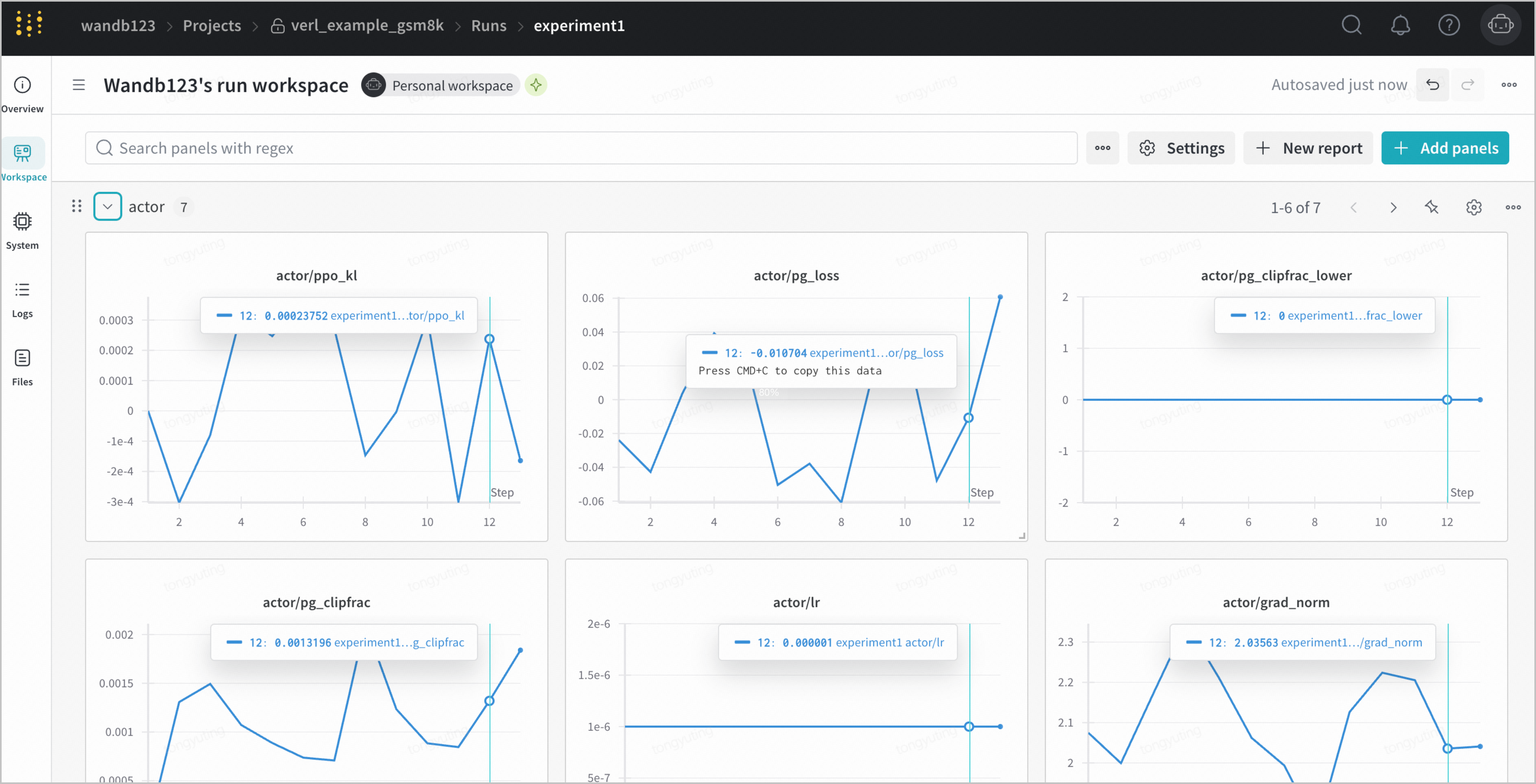
- 随后即可在 wandb 监控页面看到训练过程的指标数据。
-
使用创建的 Code Sandbox 连接 VeRL 训练
- reward_model.sandbox_fusion_url修改为创建的sandbox url+"run_code"。
- actor_rollout_ref.model.path和critic.model.path都改成容器中存放 Qwen2.5 的路径。
- data.train_files和data.val_files改成容器中存放数据集的路径。
- reward_model.reward_manager=prime表示每个 prompt 生成的多个 response 可并发执行。
- 其他参数,如reward_model.sandbox_fusion.max_concurrentsandbox的最大并发量,data.train_batch_size等等参数均可根据 sandbox实例数进行设置。详情请参见 VeRL 参数配置说明。
cd /workspace/verl
ray job submit --address="http://127.0.0.1:8265" \
--runtime-env=verl/trainer/runtime_env.yaml \
--no-wait \
-- \
python3 -m verl.trainer.main_ppo \
reward_model.sandbox_fusion.url='https://xxxxx.apigateway-cn-beijing.volceapi.com/run_code' \
reward_model.sandbox_fusion.max_concurrent=256 \
reward_model.reward_manager=prime \
algorithm.adv_estimator=gae \
data.train_files=/data/models/Eurus-2-RL-Data/train1000.parquet \
data.val_files=/data/models/Eurus-2-RL-Data/validation.parquet \
data.train_batch_size=128 \
data.max_prompt_length=512 \
data.max_response_length=512 \
data.filter_overlong_prompts=True \
data.truncation='error' \
actor_rollout_ref.model.path=/data/models/Qwen2.5-7B-Instruct-1M \
actor_rollout_ref.actor.optim.lr=1e-6 \
actor_rollout_ref.model.use_remove_padding=True \
actor_rollout_ref.actor.ppo_mini_batch_size=128 \
actor_rollout_ref.actor.ppo_micro_batch_size_per_gpu=8 \
actor_rollout_ref.actor.fsdp_config.param_offload=False \
actor_rollout_ref.actor.fsdp_config.optimizer_offload=False \
actor_rollout_ref.actor.use_kl_loss=False \
actor_rollout_ref.model.enable_gradient_checkpointing=True \
actor_rollout_ref.rollout.log_prob_micro_batch_size_per_gpu=16 \
actor_rollout_ref.rollout.tensor_model_parallel_size=4\
actor_rollout_ref.rollout.name=vllm \
actor_rollout_ref.rollout.gpu_memory_utilization=0.4 \
critic.optim.lr=1e-5 \
critic.model.use_remove_padding=True \
critic.model.path=/data/models/Qwen2.5-7B-Instruct-1M \
critic.model.enable_gradient_checkpointing=True \
critic.ppo_micro_batch_size_per_gpu=16 \
critic.model.fsdp_config.param_offload=False \
critic.model.fsdp_config.optimizer_offload=False \
algorithm.use_kl_in_reward=False \
trainer.logger=['console','wandb'] \
trainer.project_name='very_ppo' \
trainer.experiment_name='experiment_sandbox_723' \
trainer.critic_warmup=0 \
trainer.default_local_dir='/data/sandboxcheckpoints'\
trainer.n_gpus_per_node=8 \
trainer.nnodes=1 \
trainer.save_freq=20 \
trainer.test_freq=20 \
trainer.total_epochs=20
训练性能对比
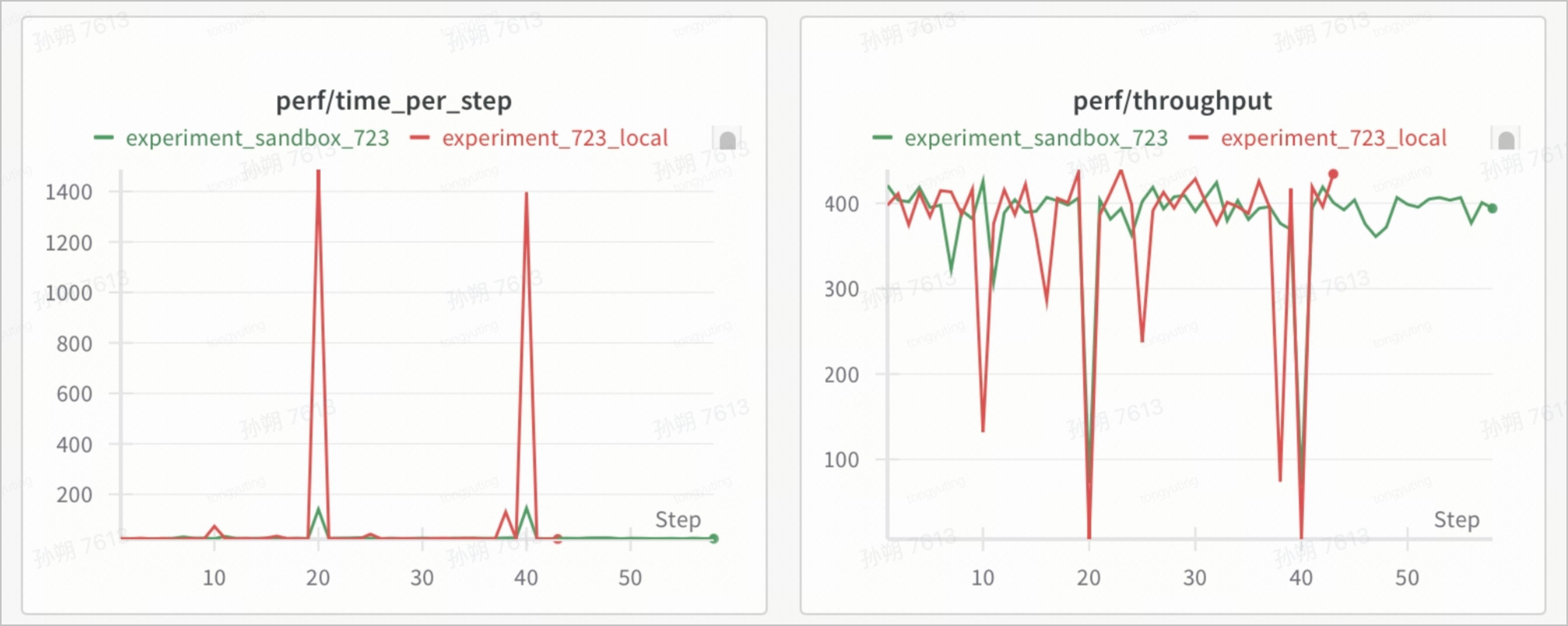
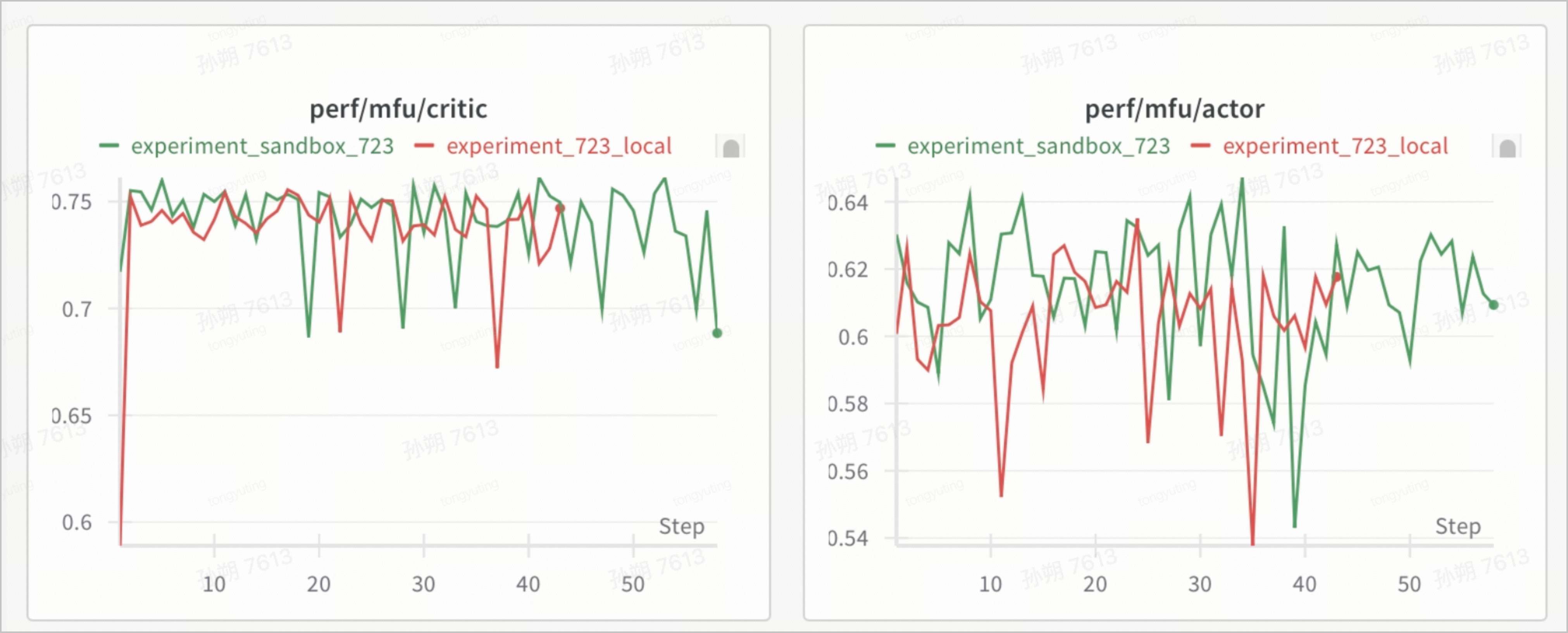
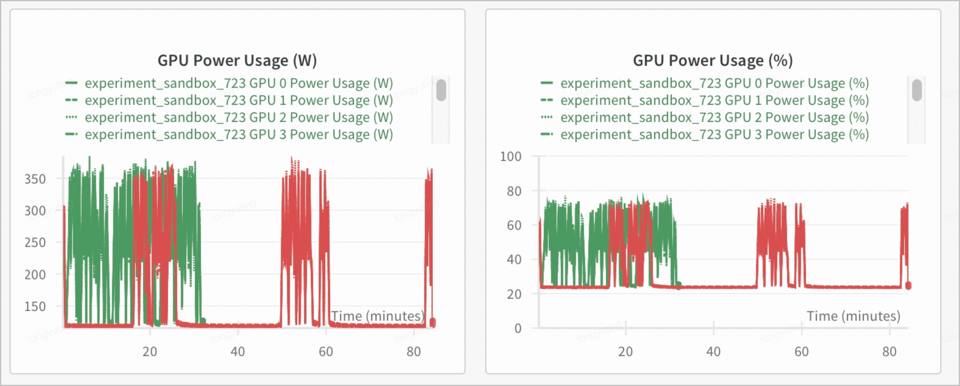
通过 wandb 监控页面查看训练过程的指标数据,查看性能对比、资源利用率等指标。相同实验设置下,FaaS 部署 Sandbox Fusion 每个 step 的训练时长相较于本地训练显著减少,吞吐量显著增加。
训练后模型能力评测
模型合并
fsdp 将不同显卡上训练的模型文件拆分显卡数量个文件,执行以下命令将 checkpoint/actor 中的模型合并为 huggingface 格式模型。
- local_dir指定为某个 checkpoint 的 actor 文件夹。
- target_dir指定为输出模型的文件夹,可指定为/data目录下任意目录以保存到 TOS 桶内。
cd /workspace/verl
python scripts/model_merger.py merge \
--backend fsdp \
--local_dir /data/checkpoints/global_step_130/actor \
--target_dir /data/models/Qwen2.5-7B-Instruct-1M-step130
模型评测
- 安装 EvalScope
git clone https://github.com/modelscope/evalscope.git
cd evalscope/
pip install -e . # 安装 Native backend# 额外选项
pip install -e '.[opencompass]' # 安装 OpenCompass backend
pip install -e '.[vlmeval]' # 安装 VLMEvalKit backend
pip install -e '.[rag]' # 安装 RAGEval backend
pip install -e '.[perf]' # 安装 模型压测模块 依赖
pip install -e '.[app]' # 安装 可视化 相关依赖
pip install -e '.[all]' # 安装所有 backends (Native, OpenCompass, VLMEvalKit, RAGEval)
- 执行数据集评测。
evalscope eval \
--model /data/models/Qwen2.5-7B-Instruct-1M-step130 \#/data/Qwen2.5-7B-Instruct-1M 更换参数可更换模型
--datasets gsm8k# humaneval # live_code_bench 更换参数可更换评测数据集
--limit 100 #从评测数据集选择的样本数
评测结果
- gsm8k Case 展示
- 分析:
- 经过在EURUS数据集上RL后 ,模型数学推理能力有明显提升,数学推理步骤逻辑更加清晰,语言更简洁,更能按照提示词要求输出答案格式。
- 当前 RL 的模型累计训练 130 steps,使用EURUS约1000条训练数据。理论上增加训练步数和使用更多的训练数据,还有进一步提升空间。
- 验证集 Case展示:
- 7 道编程题 Case(来自验证集):2道简单 + 2道中等 + 3道困难,覆盖考察点多样。
- 随着训练过程的逐步进行,模型返回的代码评分逐渐变高,体现训练策略的有效性和模型在各类编程任务上的鲁棒性。
考察点 | 题面 | 样例 | 训练过程score变化(轮数较少) |
贪心算法 | 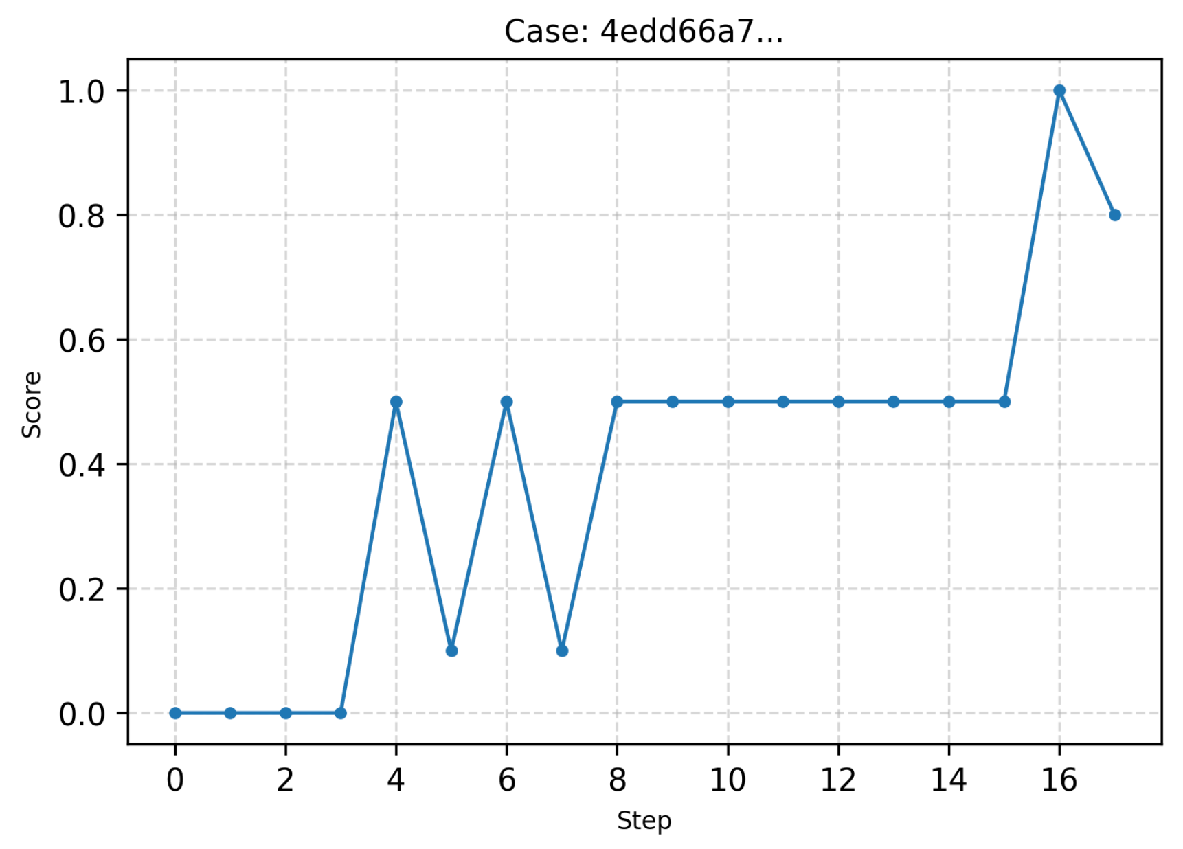 | ||
字符串模式匹配 | 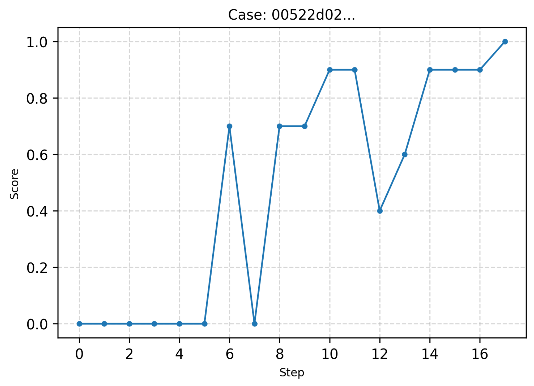 | ||
动态规划 | 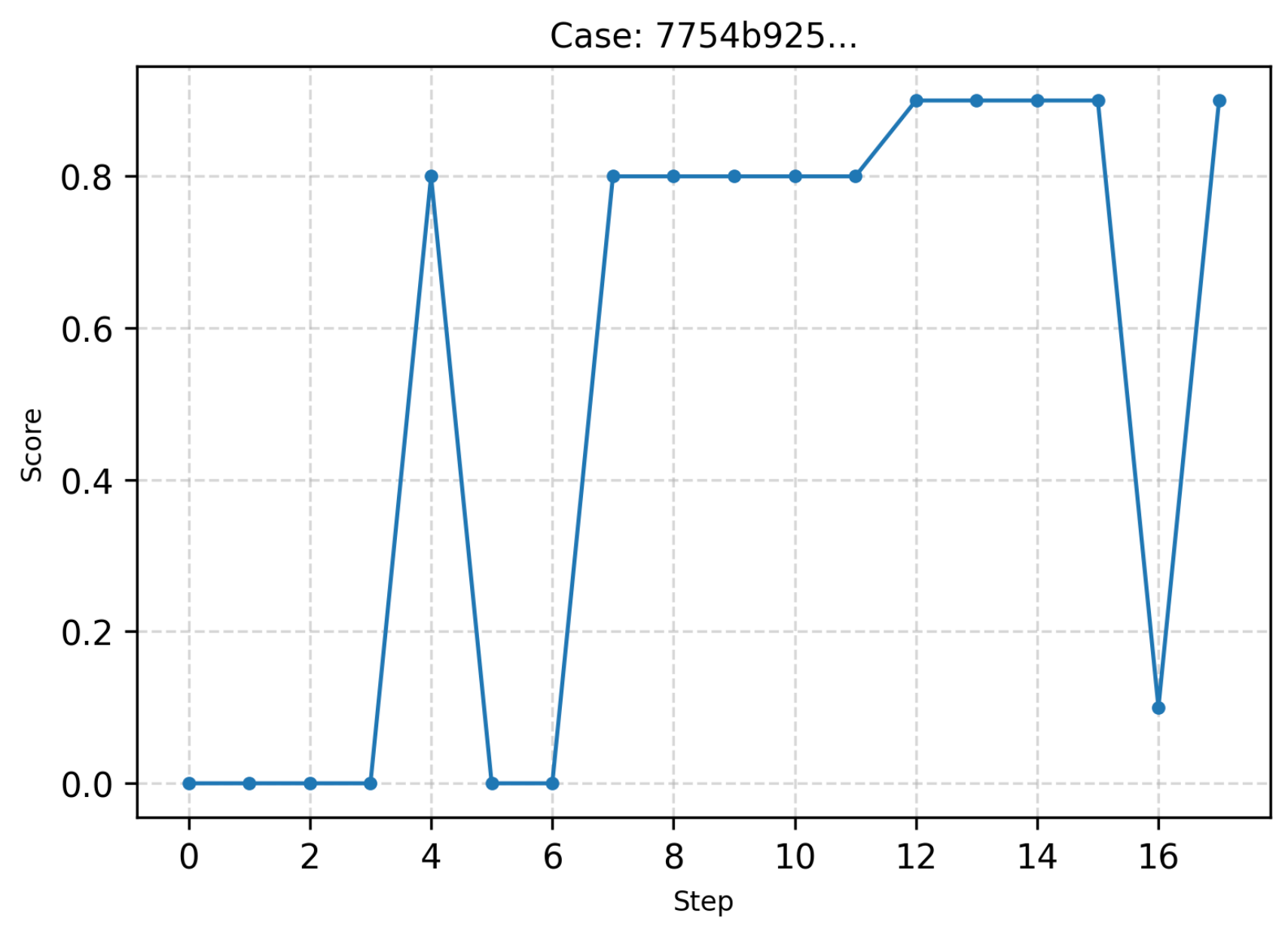 | ||
滑动窗口+前缀和 | 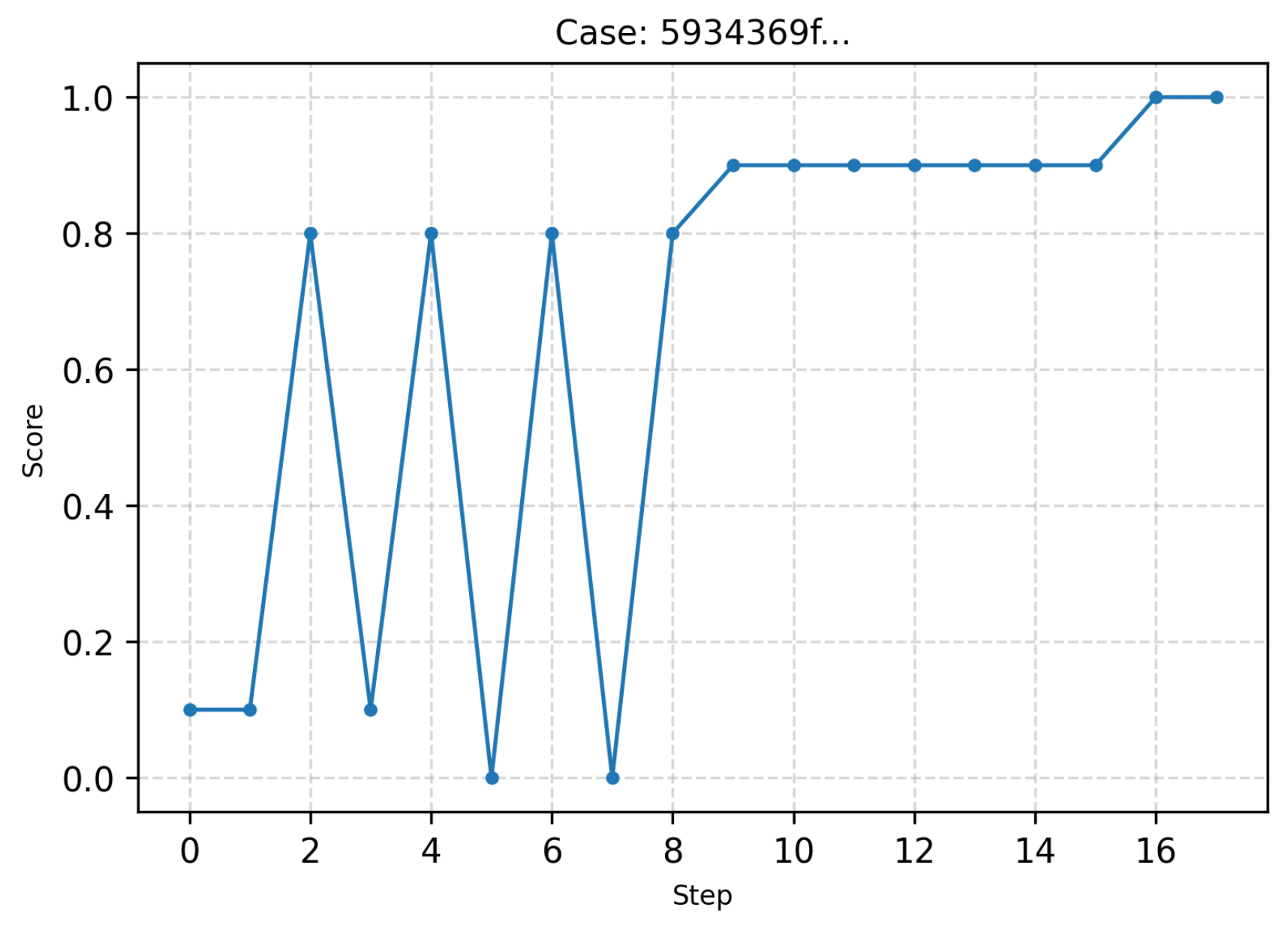 | ||
图论+动态规划 | 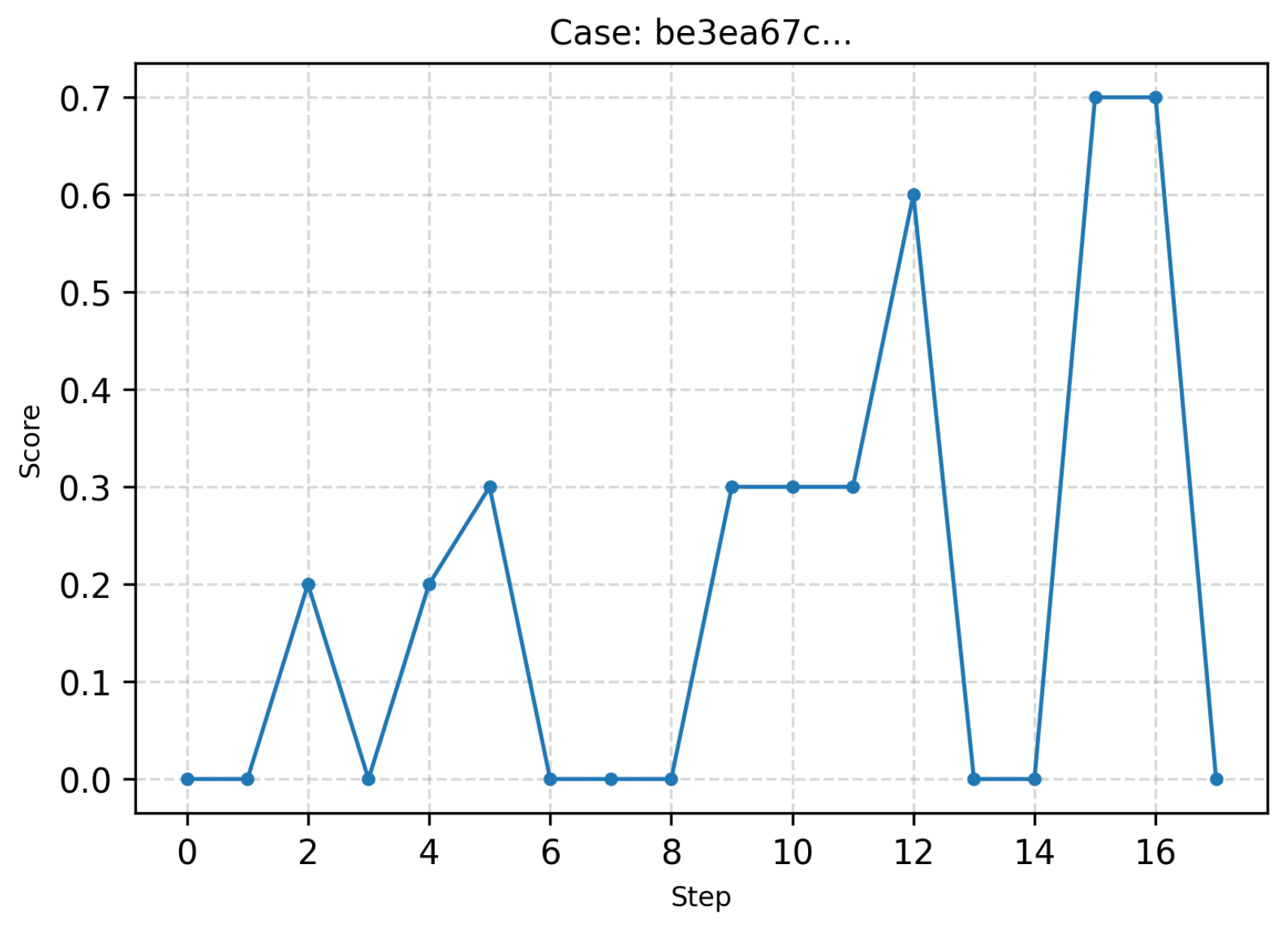 | ||
二维动态规划 | 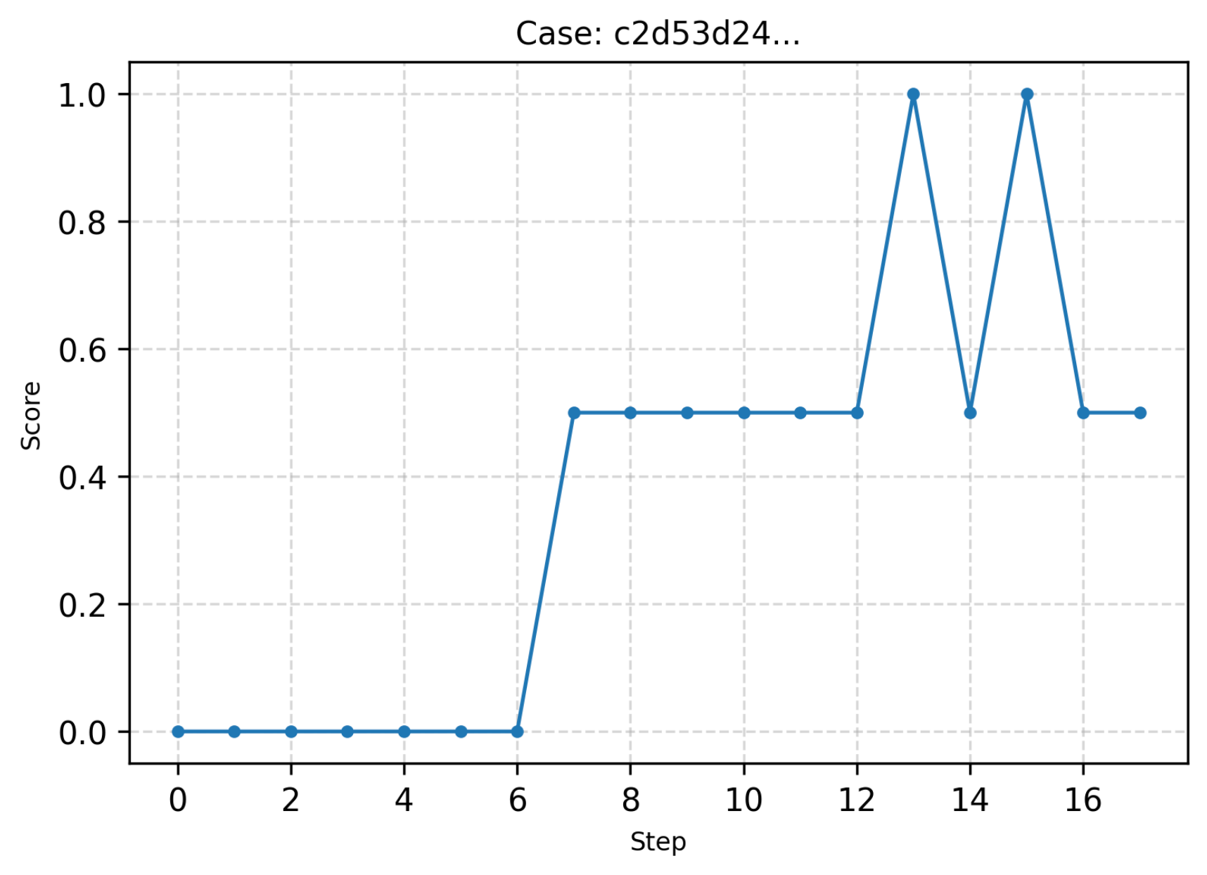 | ||
棋盘图论 | 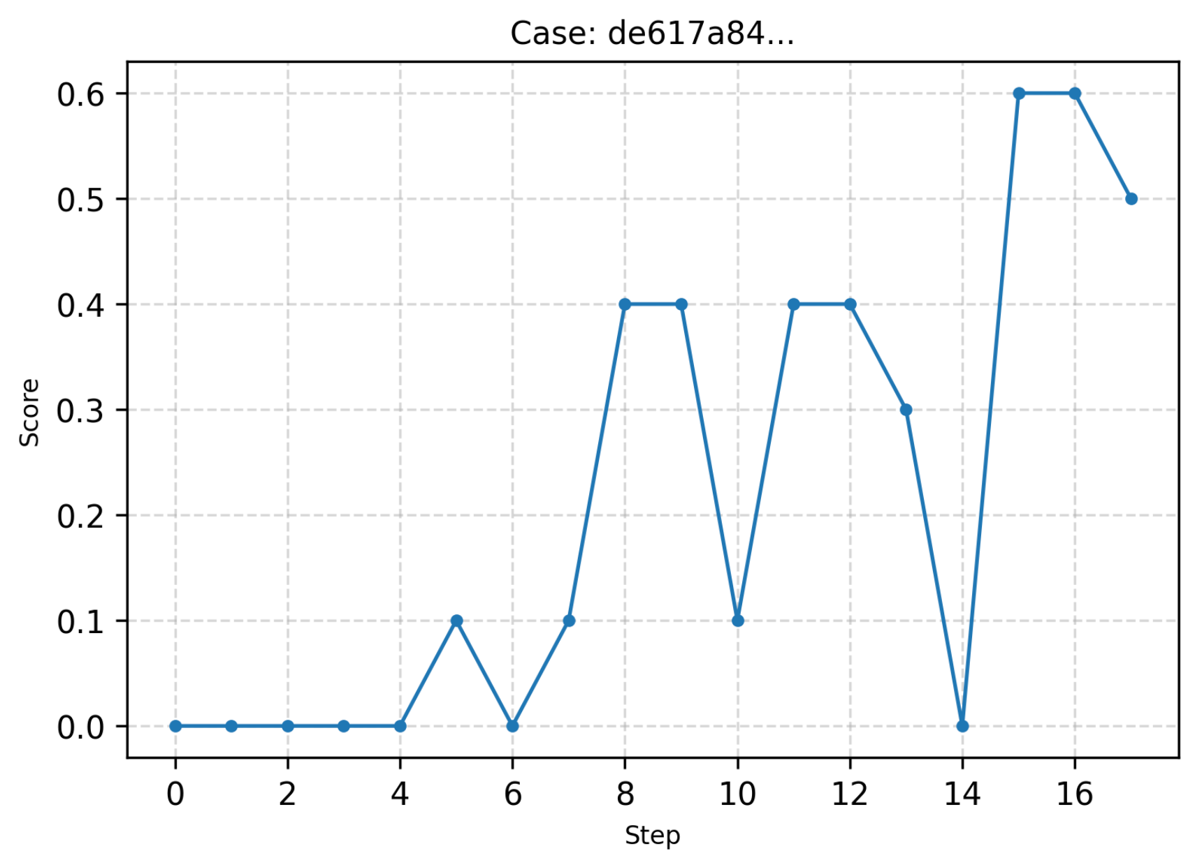 |
最近更新时间:2025.09.22 17:03:22
这个页面对您有帮助吗?
有用
有用
无用
无用